Complete Rhipicephalus microplus analysis with xnicher

Introduction

This report shows a complete xnicher workflow for modelling the ecological niche of the cattle tick Rhipicephalus microplus. Two likelihood families are compared:

• presence_only: a Gaussian ellipsoid fitted with presence points only.
• ncst: a non-central skew-t model with heavy tails and asymmetry.

The bundled dataset contains:

• rhipicephalus: coordinates and environmental values for 334 presence records and 9,784 background points inside the accessible area $M$.
• rhipicephalus_env.tif: a two-band raster with annual mean temperature (bio1, °C) and relative humidity (rh, %).

library(xnicher)
library(terra)
library(ggplot2)

# Seed for reproducibility
set.seed(123)

Load data and raster

data(rhipicephalus)

vars <- c("bio1", "rh")

# The package data frames may include an ID column from terra::extract;
# keep only the environmental variables.
env_occ  <- rhipicephalus$env_occ[, vars]
env_m    <- rhipicephalus$env_m[, vars]
coords_occ <- rhipicephalus$coords_occ
coords_m   <- rhipicephalus$coords_m

# Full two-band raster
env_stack <- rast(system.file("extdata", "rhipicephalus_env.tif",
                              package = "xnicher"))
names(env_stack) <- vars

nrow(env_occ)
#> [1] 334
nrow(env_m)
#> [1] 9784

Standardisation (z-score)

bio1 is in °C and rh is in percent. To give both variables comparable influence in the objective — especially important for ncst — we standardise using the mean and standard deviation of the background $M$.

means <- colMeans(env_m)
sds   <- apply(env_m, 2, sd)

scale_env <- function(df) {
  df <- as.data.frame(df)
  data.frame(
    bio1 = (df$bio1 - means["bio1"]) / sds["bio1"],
    rh   = (df$rh   - means["rh"])   / sds["rh"]
  )
}

env_occ_sc <- scale_env(env_occ)
env_m_sc   <- scale_env(env_m)

summary(env_occ_sc)
#>       bio1               rh         
#>  Min.   :-3.2839   Min.   :-2.7202  
#>  1st Qu.:-0.7188   1st Qu.:-0.2101  
#>  Median :-0.1895   Median : 0.1370  
#>  Mean   :-0.2324   Mean   : 0.0858  
#>  3rd Qu.: 0.2177   3rd Qu.: 0.5312  
#>  Max.   : 1.0728   Max.   : 1.5415

Train/test split

Presence records are split into 65 % for training and 35 % for evaluating predictive performance.

train_idx <- sample.int(nrow(env_occ_sc), size = floor(0.65 * nrow(env_occ_sc)))
train <- env_occ_sc[train_idx, ]
test  <- env_occ_sc[-train_idx, ]

train_coords <- coords_occ[train_idx, ]
test_coords  <- coords_occ[-train_idx, ]

nrow(train)
#> [1] 217
nrow(test)
#> [1] 117

Model fitting

Both models are fitted with 20 Sobol starts. For a final analysis, increase num_starts to 50–100.

fit_po <- optimize_niche(
  env_occ    = train,
  env_m      = NULL,
  likelihood = "presence_only",
  num_starts = 20L,
  seed       = 123L
)

assess(fit_po)
#> $flag
#> [1] "accepted_global"
#> 
#> $recommendation
#> [1] "Global optimum likely found: multiple converged starts agree closely."
#> 
#> $gap
#> [1] 5.684342e-14
#> 
#> $rel_gap
#> [1] 1.298082e-15
#> 
#> $n_converged
#> [1] 20
#> 
#> $best_loglik
#> [1] -43.79031

fit_ncst <- optimize_niche(
  env_occ    = train,
  env_m      = NULL,
  likelihood = "ncst",
  num_starts = 20L,
  seed       = 123L
)

assess(fit_ncst)
#> $flag
#> [1] "accepted_global"
#> 
#> $recommendation
#> [1] "Global optimum likely found: multiple converged starts agree closely."
#> 
#> $gap
#> [1] 7.389644e-13
#> 
#> $rel_gap
#> [1] 2.325056e-15
#> 
#> $n_converged
#> [1] 20
#> 
#> $best_loglik
#> [1] -317.8266

Information-criteria comparison

cmp <- compare_xnicher(presence_only = fit_po, ncst = fit_ncst)
cmp[, c("model", "likelihood", "df", "loglik", "AIC", "BIC", "convergence")]
#>           model    likelihood df     loglik       AIC      BIC convergence
#> 1 presence_only presence_only  5  -43.79031  97.58063 114.4801           1
#> 2          ncst          ncst  8 -316.01525 648.03049 675.0697           1

TSS on the test set

The True Skill Statistic (TSS) is computed with a background sample of the same size as the test presences.

compute_tss <- function(suit_pres, suit_bg) {
  vals <- c(suit_pres, suit_bg)
  lab  <- c(rep(1, length(suit_pres)), rep(0, length(suit_bg)))
  ok   <- is.finite(vals)
  if (sum(ok) == 0) return(c(tss = NA_real_, threshold = NA_real_))
  vals <- vals[ok]
  lab  <- lab[ok]
  np   <- sum(lab == 1)
  nb   <- sum(lab == 0)
  if (np == 0 || nb == 0) return(c(tss = NA_real_, threshold = NA_real_))
  if (nb > np) {
    set.seed(123)
    vals_bg   <- vals[lab == 0]
    vals_pres <- vals[lab == 1]
    vals_bg   <- sample(vals_bg, size = np, replace = FALSE)
    vals      <- c(vals_pres, vals_bg)
    lab       <- c(rep(1, np), rep(0, np))
    nb        <- np
  }
  thresholds <- sort(unique(vals), decreasing = TRUE)
  thresholds <- c(thresholds, min(thresholds, na.rm = TRUE) - 1)
  tss_vec <- vapply(thresholds, function(t) {
    pred <- as.integer(vals > t)
    sens <- sum(pred[lab == 1]) / np
    spec <- sum(1 - pred[lab == 0]) / nb
    sens + spec - 1
  }, numeric(1))
  best <- which.max(tss_vec)
  c(tss = tss_vec[best], threshold = thresholds[best])
}

A raster cropped to the study area is standardised with the same parameters used during training and then projected with each fitted model.

cm <- coords_m
e  <- ext(min(cm$lon) - 5, max(cm$lon) + 5,
          min(cm$lat) - 5, max(cm$lat) + 5)

env_crop <- crop(env_stack, e)
env_crop[["bio1"]] <- (env_crop[["bio1"]] - means["bio1"]) / sds["bio1"]
env_crop[["rh"]]   <- (env_crop[["rh"]]   - means["rh"])   / sds["rh"]
env_crop <- env_crop[[vars]]

# Geographic projections
suit_po   <- predict(fit_po,   env_crop, threads = 1)
suit_ncst <- predict(fit_ncst, env_crop, threads = 1)

Suitability values at test and background points are extracted. Some versions of terra keep an ID column even with ID = FALSE, so the layer name suitability is used explicitly.

v_test <- vect(test_coords, geom = c("lon", "lat"), crs = "EPSG:4326")
v_bg   <- vect(coords_m,    geom = c("lon", "lat"), crs = "EPSG:4326")

s_test_po <- terra::extract(suit_po,   v_test)$suitability
s_bg_po   <- terra::extract(suit_po,   v_bg)$suitability
s_test_nc <- terra::extract(suit_ncst, v_test)$suitability
s_bg_nc   <- terra::extract(suit_ncst, v_bg)$suitability

tss_po   <- compute_tss(s_test_po,   s_bg_po)
tss_ncst <- compute_tss(s_test_nc,   s_bg_nc)

knitr::kable(data.frame(
  model     = c("presence_only", "ncst"),
  TSS       = c(tss_po["tss"],   tss_ncst["tss"]),
  threshold = c(tss_po["threshold"], tss_ncst["threshold"]),
  row.names = NULL
), digits = 4)

model	TSS	threshold
presence_only	0.2564	0.2681
ncst	0.3333	0.4253

Iso-suitability in environmental space

bg_sample <- env_m_sc[sample.int(nrow(env_m_sc), 3000), ]

p_po <- ggplot() +
  geom_xnicher_background(bg_sample) +
  geom_xnicher_occ(env_occ_sc, colour = "black", size = 0.8, alpha = 0.4) +
  geom_xnicher_isosuitability(fit_po,
                              level = c(0.95, 0.75, 0.5, 0.25, 0.05),
                              colour = "firebrick") +
  labs(title = "presence_only: bio1 x rh",
       x = "bio1 (z-score)", y = "rh (z-score)")

p_ncst <- ggplot() +
  geom_xnicher_background(bg_sample) +
  geom_xnicher_occ(env_occ_sc, colour = "black", size = 0.8, alpha = 0.4) +
  geom_xnicher_isosuitability(fit_ncst,
                              level = c(0.95, 0.75, 0.5, 0.25, 0.05),
                              colour = "steelblue") +
  labs(title = "ncst: bio1 x rh",
       x = "bio1 (z-score)", y = "rh (z-score)")

print(p_po)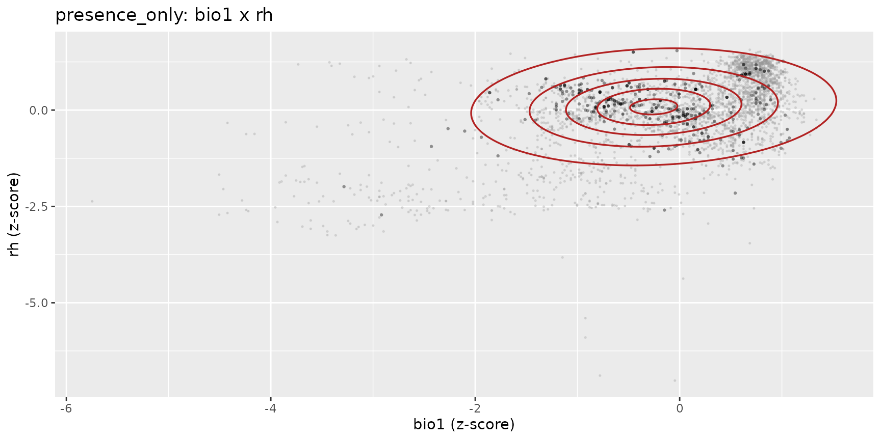

print(p_ncst)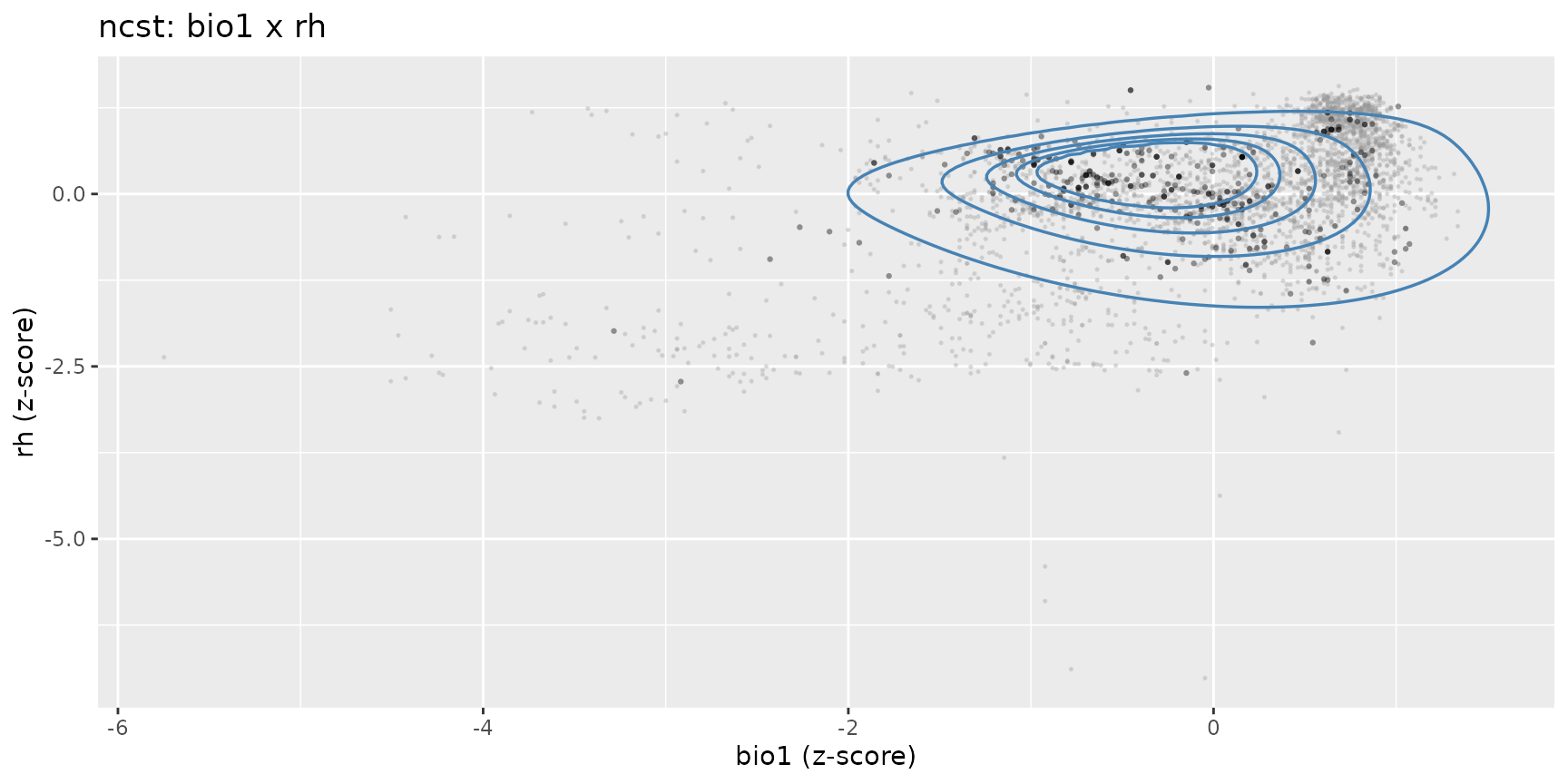

Geographic suitability maps

op <- par(mfrow = c(1, 2), mar = c(3, 3, 3, 5))

plot(suit_po, main = "presence_only: suitability",
     range = c(0, 1), col = hcl.colors(100, "YlOrRd"))
points(test_coords$lon, test_coords$lat, pch = 4, cex = 0.5, col = "blue")

plot(suit_ncst, main = "ncst: suitability",
     range = c(0, 1), col = hcl.colors(100, "YlOrRd"))
points(test_coords$lon, test_coords$lat, pch = 4, cex = 0.5, col = "blue")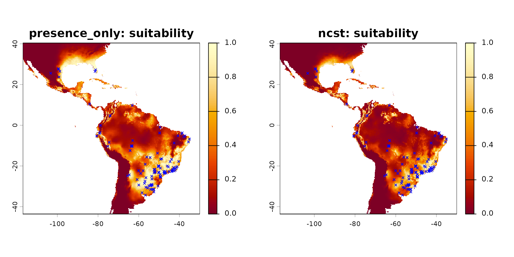

par(op)

Binary maps using the TSS threshold

suit_bin_po   <- suit_po   > tss_po["threshold"]
suit_bin_ncst <- suit_ncst > tss_ncst["threshold"]

op <- par(mfrow = c(1, 2), mar = c(3, 3, 3, 5))

plot(suit_bin_po, main = "presence_only: presence / absence",
     col = c("white", "firebrick"), legend = FALSE)
points(test_coords$lon, test_coords$lat, pch = 4, cex = 0.5, col = "blue")

plot(suit_bin_ncst, main = "ncst: presence / absence",
     col = c("white", "steelblue"), legend = FALSE)
points(test_coords$lon, test_coords$lat, pch = 4, cex = 0.5, col = "blue")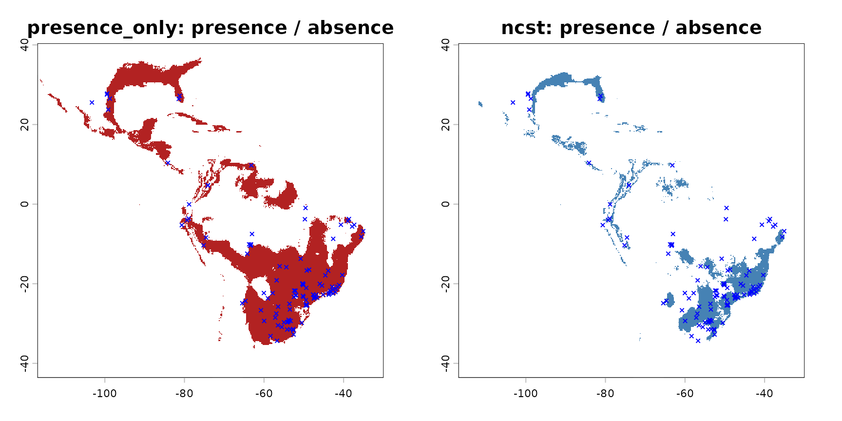

par(op)

Summary and conclusions

resumen <- data.frame(
  model         = c("presence_only", "ncst"),
  AIC           = c(AIC(fit_po),   AIC(fit_ncst)),
  BIC           = c(BIC(fit_po),   BIC(fit_ncst)),
  TSS_test      = c(tss_po["tss"], tss_ncst["tss"]),
  TSS_threshold = c(tss_po["threshold"], tss_ncst["threshold"]),
  convergence   = c(fit_po$best$convergence, fit_ncst$best$convergence)
)

knitr::kable(resumen, digits = 4)

model	AIC	BIC	TSS_test	TSS_threshold	convergence
presence_only	97.5806	114.4801	0.2564	0.2681	1
ncst	648.0305	675.0697	0.3333	0.4253	1

• The presence_only model has a much lower BIC/AIC, indicating a more parsimonious fit for this dataset.
• The ncst model reaches a slightly higher TSS (greater discriminative power on the test set), but the gain does not compensate for the extra parameter penalty.
• The R. microplus presence cloud is fairly symmetric in standardised environmental space, so the Gaussian ellipsoid already describes the niche well. The additional skewness / heavy-tail flexibility of ncst does not improve the likelihood enough to be preferred.

If the goal is spatial prediction, ncst may still be useful when tested with more starts or when robustness to heavy tails is required. If the goal is parsimonious model selection, presence_only is the best choice with these data.