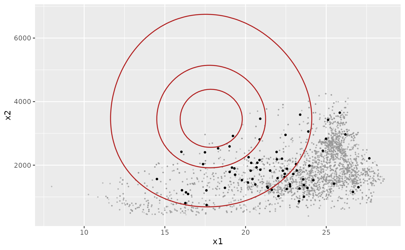
Iso-suitability contour layer derived from a fitted xnicher model — geom_xnicher

Builds a self-contained ggplot2 layer that draws iso-suitability contours, i.e. level sets $S(x) = c$ of the fitted niche suitability function over a 2-D environmental grid. Unlike geom_xnicher_ellipse, which traces analytical ellipses and is therefore tied to the Gaussian (multivariate normal) niche geometry, this layer evaluates the model's actual suitability function on a grid and contours the result. It works correctly for any likelihood family supported by optimize_niche(), including the skew-normal families ("skew_normal" and "skew_normal_weighted") where the iso-suitability sets are not ellipses.

Usage

geom_xnicher_isosuitability(
  model,
  level = c(0.95, 0.5, 0.05),
  n = 121L,
  expand = 0.1,
  linewidth = 0.6,
  colour = "firebrick",
  ...
)

Arguments

model: A xnicher object with length(model$var_names) == 2 (or, for legacy fits without var_names, a 2-D fit).
level: Numeric vector of contour levels in $(0, 1]$. Default c(0.95, 0.5, 0.05).
n: Integer grid resolution per axis. Default 121 (i.e. a 121 x 121 grid). Higher gives smoother contours at proportionally higher cost.
expand: Numeric scalar in $(0, 1)$. The grid spans $\mu \pm (1 + \mathtt{expand}) \cdot k \cdot \sigma_{\mathrm{eff}}$ along each axis, where $k = 4$ matches the typical 4-sigma support of a Gaussian niche and $\sigma_{\mathrm{eff}}$ is the marginal standard deviation. Default 0.1 (10% padding).
linewidth: Path linewidth (or size on ggplot2 < 3.4.0).
colour: Path colour.
...: Additional fixed parameters passed to geom_contour.

Value

A ggplot2 layer.

Why "iso-suitability" and not just "ellipse"

For a Gaussian niche, the suitability function $S(x) \propto \exp(-\frac{1}{2} (x-\mu)^\top \Sigma^{-1} (x-\mu))$ has elliptical level sets; the family of contours $S(x) = c$ traces nested concentric ellipses around $\mu$. For a skew-normal niche $S(x) \propto \phi_2(x; \mu, \Sigma) \, \Phi(\alpha^\top \omega^{-1} (x - \mu))$ the $\Phi(\cdot)$ factor breaks the ellipse symmetry: contours bunch on the side that $\alpha$ pulls suitability toward, and stretch on the opposite side. The contour at level $c$ is still a closed curve enclosing high-suitability environments, but it is no longer an ellipse and has no closed-form parameterisation. The only honest visualisation is to evaluate $S(x)$ on a dense 2-D grid and contour the result – which is exactly what this layer does.

Suitability normalisation

Suitability is always normalised so that $S(\mu^*) = 1$ at the modal centre: for the Gaussian families that is the centre $\mu$; for the skew-normal it is the location parameter $\mu$ from the SN $(\mu, \Sigma, \alpha)$ parameterisation (Azzalini & Capitanio 1999), which is generally not the global suitability maximum but is a well-defined reference point. The contour level level = 0.5 therefore always means "regions where the niche is at least 50% as suitable as the reference centre".

References

Azzalini, A. & Capitanio, A. (1999). Statistical applications of the multivariate skew normal distribution. Journal of the Royal Statistical Society, Series B, 61(3), 579–602.

Examples

# \donttest{
  library(ggplot2)
  fit <- optimize_niche(
    env_occ    = example_env_occ_2d,
    env_m      = example_env_m_2d,
    num_starts = 5L,
    likelihood = "skew_normal_weighted"
  )
  ggplot() +
    geom_xnicher_background(example_env_m_2d) +
    geom_xnicher_occ(example_env_occ_2d) +
    geom_xnicher_isosuitability(fit)

# }