Virtual species in a real bioregion

This vignette closes the simulation loop: simulate a known niche-evolution process inside a real accessible area, then recover it. It is the fastest way to learn what the joint phylo-niche model can and cannot identify before analysing empirical clades.

The workflow:

Take a real bioregion polygon as the shared accessible area $M$ (One Earth Bioregions Framework via oneearthr).
Build a plausible two-dimensional environmental space over $M$ .
Evolve a virtual clade’s niche under BM, OU and the independent-species null.
Draw occurrences with virtual_species_occurrences() and rebuild the posterior modes with niche_multistart().
Compare recovered niches against the truth — including which species land on identifiability boundaries.

library(arfun)
library(ape)
set.seed(42)

1. A real accessible area

We use the Andean Mountain Forests & Valleys bioregion (NT11) — home to the hummingbird clades that motivated this machinery. The rasterized NT11 footprint (0.25° cell centres) ships inside the package (inst/extdata/, extracted via oneearthr + terra), so the vignette needs no spatial dependencies.

coords <- as.matrix(readRDS(system.file("extdata", "nt11_points.rds",
                                        package = "arfun")))
plot(coords, pch = ".", cex = 3, col = "steelblue", asp = 1,
     main = "NT11 -- Andean Mountain Forests & Valleys",
     xlab = "lon", ylab = "lat")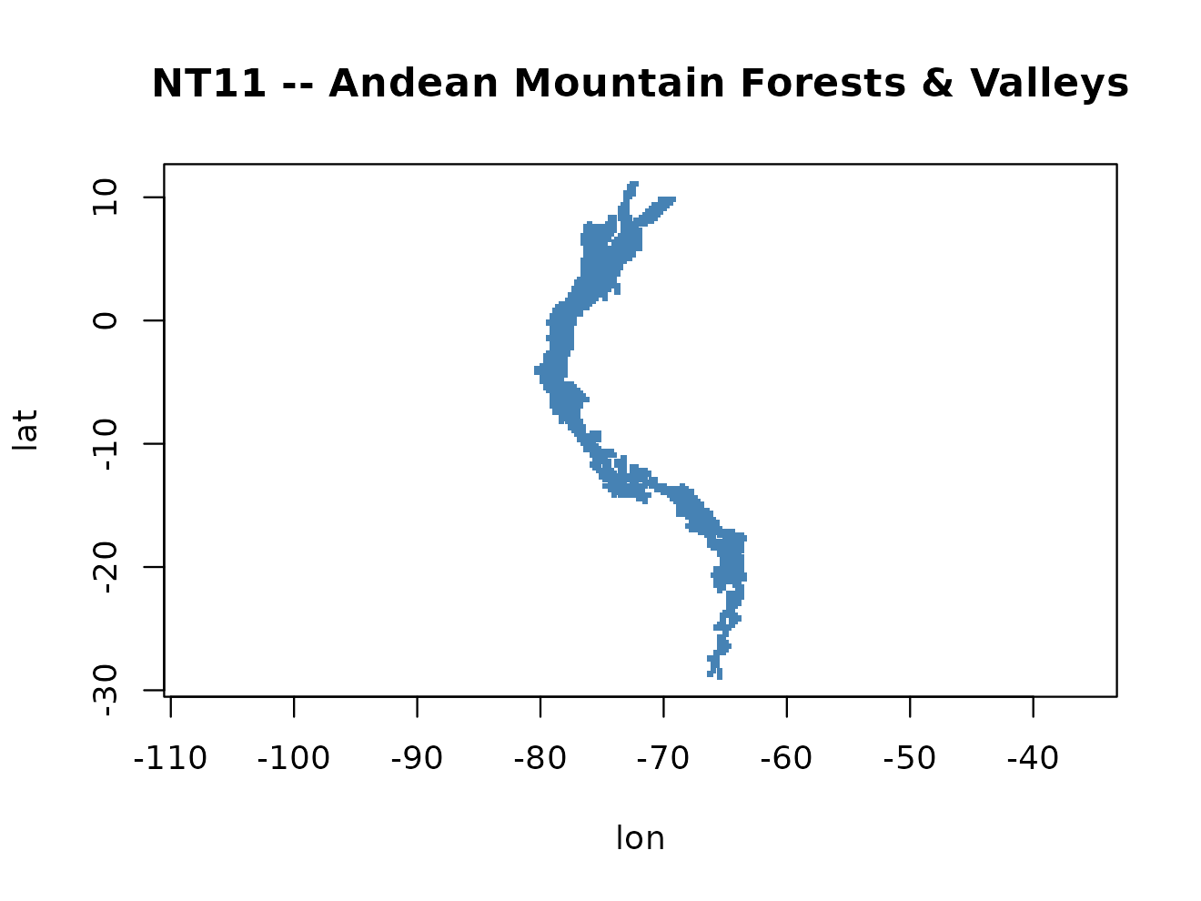

nrow(coords)
#> [1] 1259

2. A plausible environmental space over $M$

Real clade pipelines extract ERA5/WorldClim values at each cell. Here we synthesise two axes as smooth functions of geography – an elevation-flavoured temperature axis and a precipitation axis with longitudinal structure – then standardise. What matters is that $M$ is real: its holes, corridor structure and extent are the bioregion’s own.

lon <- scale(coords[, 1])[, 1]
lat <- scale(coords[, 2])[, 1]
temp <- -lat + 0.4 * lon + rnorm(length(lon), 0, 0.25)
prec <- 0.8 * lon - 0.3 * lat + rnorm(length(lon), 0, 0.35)
env_M <- scale(cbind(temp, prec))
colnames(env_M) <- c("bio1", "bio12")

plot(env_M, pch = ".", col = "grey70",
     main = "Environmental space of M")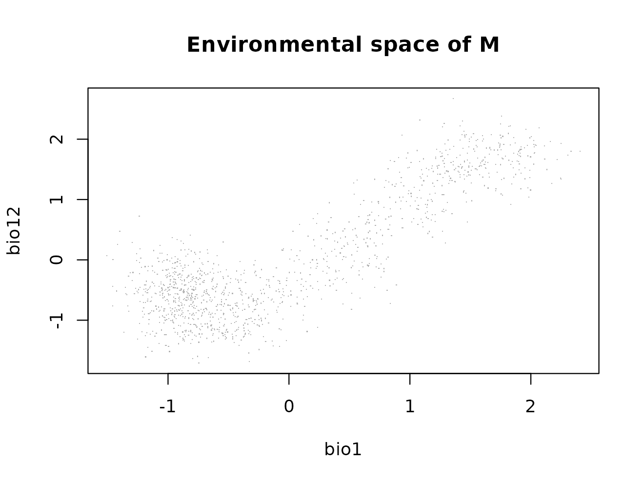

3. Evolve a virtual clade

Six virtual species evolving under each process. simulate_niche_evolution() returns the true per-species $(\mu, \sigma, \rho)$ in exactly the parameterization the joint models estimate.

tree <- rtree(6, tip.label = paste0("vsp", 1:6))
tree$edge.length <- tree$edge.length / max(ape::vcv(tree))  # unit height

truths <- lapply(c("bm", "ou", "null"), function(pr)
  simulate_niche_evolution(tree, process = pr,
                           mu_anc = c(0, 0),
                           log_sigma_anc = log(c(0.45, 0.45)),
                           rate_mu = c(0.35, 0.35),
                           rate_log_sigma = c(0.3, 0.3),
                           rate_rho = 0.4,
                           alpha = c(2, 2, 2), seed = 42))
names(truths) <- c("bm", "ou", "null")

# draw occurrences: 120 per species, shared accessible area
occ_list <- lapply(truths, function(tr)
  lapply(seq_along(tree$tip.label), function(s)
    virtual_species_occurrences(env_M, mu = tr$mu[s, ],
                                sigma = tr$sigma[s, ], rho = tr$rho[s],
                                n_occ = 120)))
for (pr in names(occ_list)) names(occ_list[[pr]]) <- tree$tip.label

# the SAME background rows for every species -- never independent draws
bg_list <- lapply(tree$tip.label, function(s) env_M)
names(bg_list) <- tree$tip.label

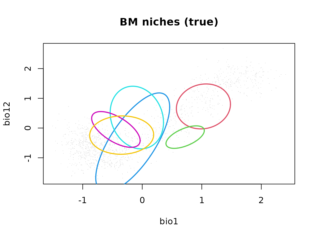
# 68% ellipse of a bivariate normal niche, no extra dependency
niche_ellipse <- function(mu, sigma, rho, level = 0.68, n = 100) {
  Sig <- matrix(c(sigma[1]^2, rho * prod(sigma),
                  rho * prod(sigma), sigma[2]^2), 2, 2)
  L <- t(chol(Sig))
  th <- seq(0, 2 * pi, length.out = n)
  t(mu + sqrt(qchisq(level, 2)) * (L %*% rbind(cos(th), sin(th))))
}

tr <- truths$bm
plot(env_M, pch = ".", col = "grey85",
     main = "BM niches (true)", xlab = "bio1", ylab = "bio12")
for (s in 1:6) {
  lines(niche_ellipse(tr$mu[s, ], tr$sigma[s, ], tr$rho[s]),
        col = s + 1, lwd = 2)
}

4. Recover: multistart MAP

fits <- lapply(names(occ_list), function(pr) {
  d <- prepare_phylo_niche_data(occ_list[[pr]], bg_list, tree)
  niche_multistart(d, "noncentered_bounded", n_starts = 12,
                   seed = 7, verbose = FALSE)
})
names(fits) <- names(occ_list)
fits$bm
#> niche_multistart (bnd)
#>   species: 6 | masked: 0 
#>   map lp: -4045.27 | solutions: 12

5. Truth vs recovery

recover_traits <- function(fit) {
  # unpack the MAP back to (mu, sigma, rho) per species
  data <- prepare_phylo_niche_data(occ_list$bm, bg_list, tree)
  rep <- fit$boundary  # per-species sigma1, sigma2, rho at the MAP
  rep[, c("species", "sigma1", "sigma2", "rho")]
}

for (pr in c("bm", "ou", "null")) {
  tr <- truths[[pr]]; rec <- fits[[pr]]$boundary
  cat("\n--- process:", pr, "---\n")
  print(data.frame(
    species = rec$species,
    sigma_true = round(apply(tr$sigma, 1, min), 3),
    sigma_map  = round(pmin(rec$sigma1, rec$sigma2), 3),
    rho_true   = round(tr$rho, 2),
    rho_map    = round(rec$rho, 2),
    flag       = rec$flag))
}
#> 
#> --- process: bm ---
#>      species sigma_true sigma_map rho_true rho_map flag
#> vsp1    vsp1      0.301     0.271     0.10    0.38   ok
#> vsp4    vsp4      0.213     0.204     0.57    0.60   ok
#> vsp6    vsp6      0.411     0.410     0.71    0.69   ok
#> vsp2    vsp2      0.297     0.314    -0.15   -0.20   ok
#> vsp3    vsp3      0.270     0.256    -0.62   -0.46   ok
#> vsp5    vsp5      0.356     0.358     0.02    0.08   ok
#> 
#> --- process: ou ---
#>      species sigma_true sigma_map rho_true rho_map flag
#> vsp1    vsp1      0.328     0.297     0.00    0.10   ok
#> vsp4    vsp4      0.249     0.248     0.40    0.55   ok
#> vsp6    vsp6      0.428     0.401     0.51    0.41   ok
#> vsp2    vsp2      0.369     0.374    -0.06    0.13   ok
#> vsp3    vsp3      0.347     0.400    -0.41   -0.48   ok
#> vsp5    vsp5      0.376     0.505     0.13   -0.11   ok
#> 
#> --- process: null ---
#>      species sigma_true sigma_map rho_true rho_map flag
#> vsp1    vsp1      0.516     0.536     0.17    0.18   ok
#> vsp4    vsp4      0.436     0.448    -0.02    0.19   ok
#> vsp6    vsp6      0.252     0.337    -0.06    0.03   ok
#> vsp2    vsp2      0.289     0.297     0.25    0.32   ok
#> vsp3    vsp3      0.427     0.393     0.58    0.51   ok
#> vsp5    vsp5      0.242     0.242    -0.26   -0.21   ok

6. Masking a virtual microendemic

Species whose occurrences occupy only a handful of environmental cells cannot identify a 2-D ellipse – the presence-only likelihood is unbounded as $\sigma \to 0$ . The recommended treatment is masking: keep the species in the phylogenetic prior but drop its likelihood, so the model predicts its niche from its relatives. The observed cluster then becomes a held-out validation target.

# crush vsp1 down to a microendemic: resample only 3 unique cells
occ_m <- occ_list$bm
mu_m <- truths$bm$mu[1, ]
d2 <- colSums((t(env_M) - mu_m)^2)
few <- order(d2)[1:3]
occ_m$vsp1 <- env_M[few, , drop = FALSE]

d_mask <- prepare_phylo_niche_data(occ_m, bg_list, tree,
                                   mask_species = "vsp1")
fit_mask <- niche_multistart(d_mask, "noncentered_bounded",
                             n_starts = 12, seed = 7, verbose = FALSE)
fit_mask$boundary
#>      species    sigma1    sigma2        rho emp_sd_min n_occ n_cells masked
#> vsp1    vsp1 0.2463694 0.3910682  0.4612659         NA     0       0   TRUE
#> vsp4    vsp4 0.2034516 0.2621467  0.5980811  0.1621532   120      46  FALSE
#> vsp6    vsp6 0.4085330 1.4057561  0.6863395  0.3745909   120     108  FALSE
#> vsp2    vsp2 0.3138647 0.7285104 -0.1884733  0.3461012   120     102  FALSE
#> vsp3    vsp3 0.2558391 0.3415626 -0.4599025  0.2544281   120      96  FALSE
#> vsp5    vsp5 0.3580296 0.4070837  0.0796858  0.2998985   120     105  FALSE
#>        flag
#> vsp1 masked
#> vsp4     ok
#> vsp6     ok
#> vsp2     ok
#> vsp3     ok
#> vsp5     ok

vsp1 carries flag "masked": no likelihood contribution, but the phylogenetic prior still predicts a finite niche – compare its sigma1/sigma2 against the true value used to simulate it.

Reading the boundary flags

flag	meaning
`ok`	interior optimum
`masked`	excluded from the likelihood, predicted by the prior
`at_floor`	$\sigma$ pinned at `sigma_floor` – check `n_cells` before calling it microendemic
`rho_at_cap`	sliver-like ellipse, $\\|\rho\\| \to$ cap
`sigma_huge`	nearly uniform niche over $M$
`few_cells`	narrow niche with < 15 unique cells – candidate for masking

The empirical pipeline adds one more diagnostic – whether the union of the shared background covers each species’ cluster – to separate real microendemism from background-sampling holes (see ?prepare_phylo_niche_data and ?shared_background_sample).