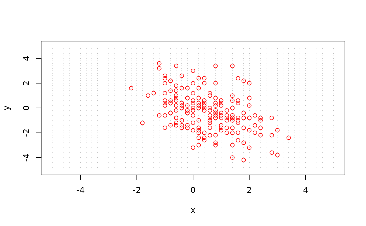
Sample occurrence points for a virtual species

Draws occurrence coordinates from the niche intensity over an environmental domain — the generative process assumed by the Jetz-and-Styles-style likelihood used in nicherbayes: intensity \(\propto \exp(-0.5\,q^2(x))\) truncated to the domain. An optional detection layer thins the draws through [probability_detection()].

Usage

virtual_species_occurrences(
  env,
  mu,
  sigma,
  rho = 0,
  n_occ,
  ctil = NULL,
  pd = 1
)

Arguments

env

Numeric matrix \(n \times p\): the environmental domain (e.g., a grid over the accessible area M).

mu

Niche centre, length \(p\).

sigma

Covariance matrix \(p \times p\) or per-axis sds (with rho).

rho

Correlation, used when sigma is a vector.

n_occ

Number of occurrences to draw.

ctil, pd

Optional detection-layer parameters. When ctil is NULL (default) occurrences are drawn with probability proportional to the niche intensity only (pure J&S process).

Value

A matrix with n_occ rows and \(p\) columns of sampled environmental coordinates.

Details

Without the detection layer this is exactly the process simulated by the recovery harness in arfun-paper-scripts (11_sim_recovery.R): occurrence intensity proportional to the niche kernel over the shared domain. With ctil/pd set, each candidate point is kept with probability probability_detection(x) — a detection-thinned variant useful for realistic virtual-species benchmarks.

Examples

env <- as.matrix(expand.grid(x = seq(-5, 5, 0.2), y = seq(-5, 5, 0.2)))
occ <- virtual_species_occurrences(env, mu = c(0.5, -0.3),
                                 sigma = c(1, 1.4), rho = -0.4,
                                 n_occ = 200)
plot(env, pch = ".", col = "grey"); points(occ, col = "red")