Round trip: evolving and reconstructing a fundamental niche
Source:vignettes/niche-roundtrip.Rmd
niche-roundtrip.RmdThis vignette does the full round trip in the idealized case where the fundamental niche itself is observed: a niche with five evolving parameters – centroid , log tolerances , and correlation – drifts by Brownian motion along a ten-species tree, generates occurrences, and is then reconstructed from the occurrences alone, including the internal nodes. The point is to see, parameter by parameter, what the evolutionary process looks like forward in time and what the reconstruction recovers backward.
The honest-scope box first: occurrences here are drawn directly from
the fundamental response over a shared, fully accessible environmental
domain – the oracle case of the paper’s Level-1/2 separation. The harder
case, where each species sees only its own accessible area
and ignoring
manufactures a spurious basal niche shift, is the M-structured null
benchmark (see validation/mnull/ in the paper repo).
1. A ten-species tree
tr <- rtree(10, tip.label = paste0("sp", 1:10))
tr$edge.length <- tr$edge.length / max(node.depth.edgelength(tr))
plot(tr, main = "simulated clade (unit height)"); axisPhylo()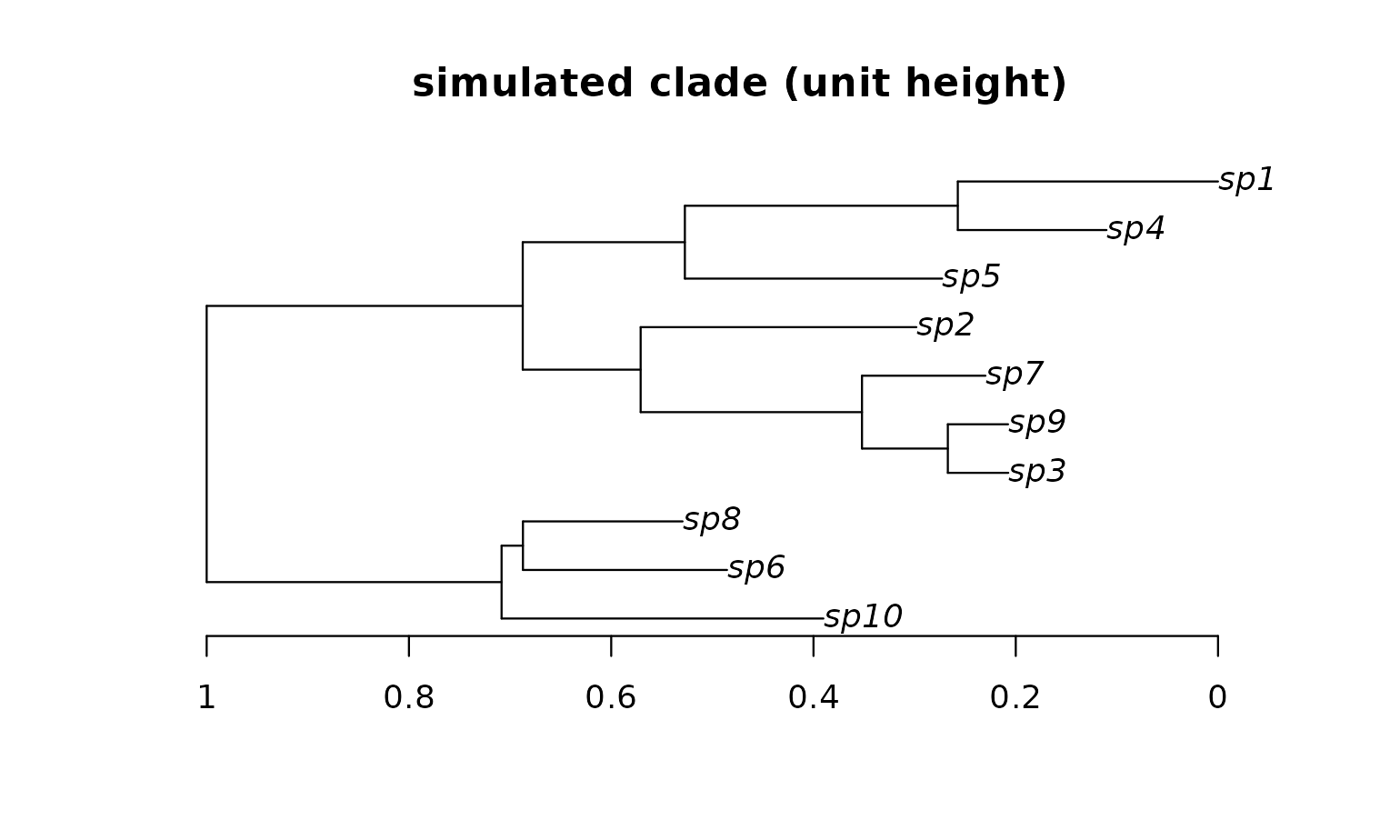
S <- length(tr$tip.label); P <- 2L2. Forward trip: the niche evolves
All five niche parameters evolve as independent Brownian motions from
a root state. We traverse the tree edge by edge – the same transition
rule simulate_niche_evolution() uses under
process = "bm",
– but keep the value at every node so the full trait history is
visible, not just the tips.
truth_anc <- list(mu = c(0, 0), ls = log(c(0.5, 0.5)), zr = 0)
rates     <- list(mu = c(0.5, 0.5), ls = c(0.4, 0.4), zr = 0.5)

evolve_bm <- function(tree, anc, rates) {
  edge <- tree$edge; el <- tree$edge.length
  n_tot <- length(tree$tip.label) + tree$Nnode
  val <- list(mu = matrix(NA_real_, n_tot, 2),
              ls = matrix(NA_real_, n_tot, 2),
              zr = matrix(NA_real_, n_tot, 1))
  val$mu[S + 1, ] <- anc$mu; val$ls[S + 1, ] <- anc$ls
  val$zr[S + 1, ] <- anc$zr
  for (e in order(edge[, 1])) {              # parents precede children
    pa <- edge[e, 1]; ch <- edge[e, 2]; t <- el[e]
    for (b in names(val))
      val[[b]][ch, ] <- val[[b]][pa, ] +
        rnorm(ncol(val[[b]]), 0, sqrt(rates[[b]] * t))
  }
  val
}

node_val <- evolve_bm(tr, truth_anc, rates)
depth <- node.depth.edgelength(tr)           # time from root, tips=1

# tip-level truth, natural scale
true_mu    <- node_val$mu[1:S, ]
true_sigma <- exp(node_val$ls[1:S, ])
true_rho   <- tanh(node_val$zr[1:S, ])
par(mfrow = c(2, 3), mar = c(3.2, 3.2, 2.2, 0.6))
panels <- list(list(node_val$mu[, 1], expression(mu[1])),
               list(node_val$mu[, 2], expression(mu[2])),
               list(node_val$ls[, 1], expression(log~sigma[1])),
               list(node_val$ls[, 2], expression(log~sigma[2])),
               list(node_val$zr[, 1], expression(z[rho])))
for (pn in panels) {
  x <- pn[[1]]
  plot(depth, x, pch = ifelse(seq_along(x) <= S, 19, 21),
       col = "grey30", xlab = "time (root -> tip)", ylab = pn[[2]],
       main = paste("true BM trajectory:", pn[[2]]))
  for (e in seq_len(nrow(tr$edge)))
    segments(depth[tr$edge[e, 1]], x[tr$edge[e, 1]],
             depth[tr$edge[e, 2]], x[tr$edge[e, 2]], col = "grey60")
  points(depth, x, pch = ifelse(seq_along(x) <= S, 19, 21),
         col = "grey30")
}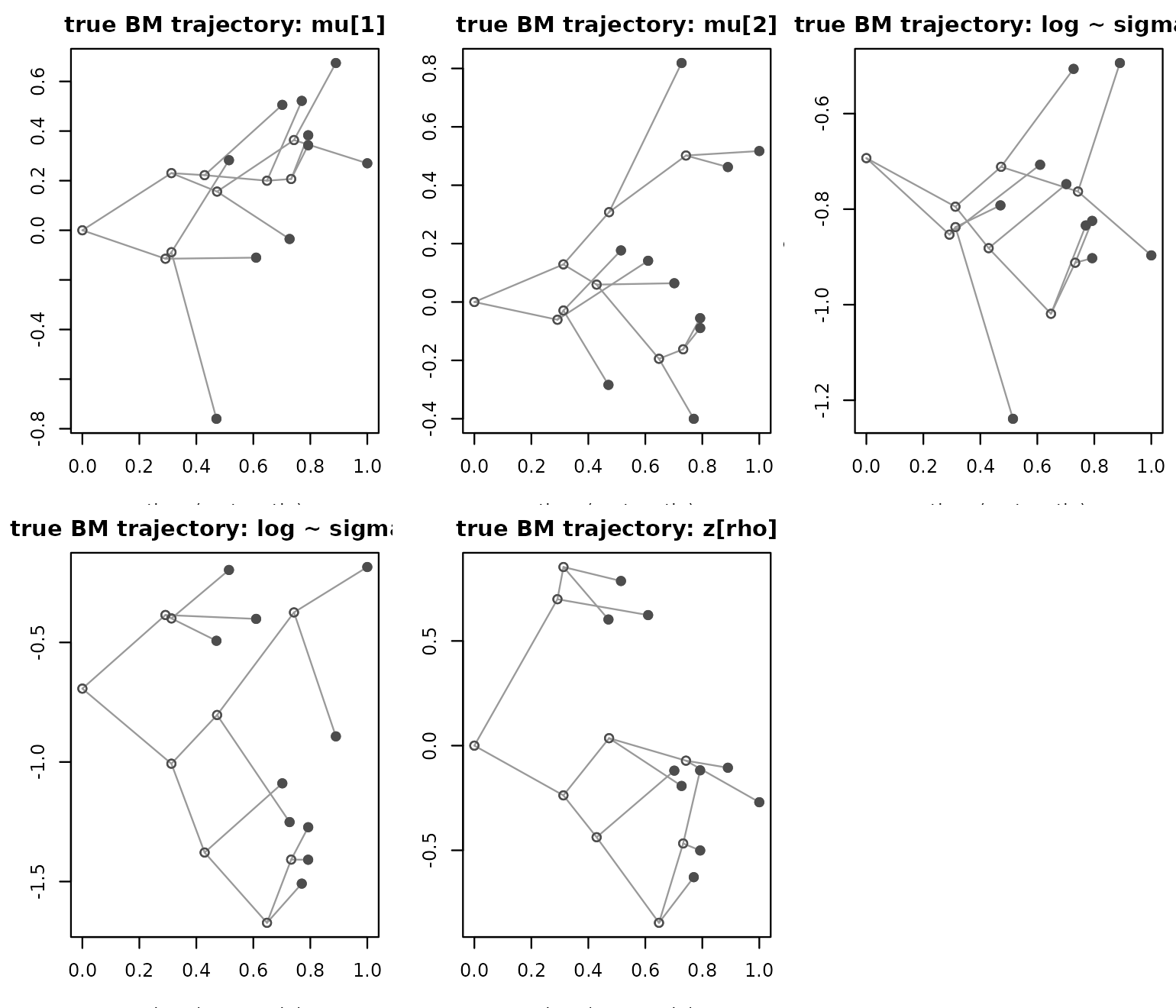
Each line segment is one branch of the tree; dots are tips, open circles internal nodes. This is what “the fundamental niche evolves” concretely means in the model: five Brownian paths sharing one topology.
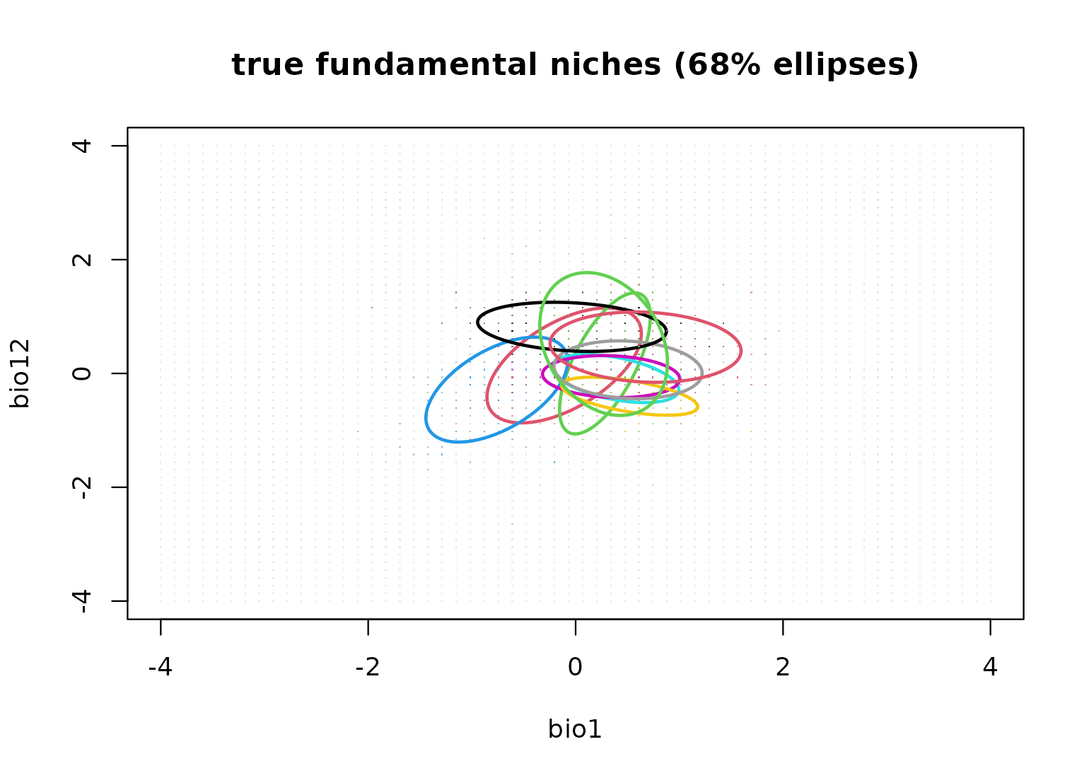
3. Occurrences from the fundamental niche
The accessible domain is a dense environmental grid – every species sees the same domain, so there is no accessibility structure to confound. Occurrences are sampled proportional to the niche intensity (Jimenez & Soberon weighting over the domain).
g <- expand.grid(bio1 = seq(-4, 4, len = 60),
                 bio12 = seq(-4, 4, len = 60))
env_grid <- as.matrix(g)
occ_list <- lapply(seq_len(S), function(s)
  virtual_species_occurrences(env_grid, mu = true_mu[s, ],
                              sigma = true_sigma[s, ],
                              rho = true_rho[s], n_occ = 150))
names(occ_list) <- tr$tip.label

# shared background sample: the SAME rows for every species
bg <- env_grid[sample.int(nrow(env_grid), 2000), ]
bg_list <- lapply(tr$tip.label, function(s) bg)
names(bg_list) <- tr$tip.label
niche_ellipse <- function(mu, sigma, rho, level = 0.68, n = 120) {
  Sig <- matrix(c(sigma[1]^2, rho * prod(sigma),
                  rho * prod(sigma), sigma[2]^2), 2, 2)
  L <- t(chol(Sig))
  th <- seq(0, 2 * pi, length.out = n)
  t(mu + sqrt(qchisq(level, 2)) * (L %*% rbind(cos(th), sin(th))))
}
plot(env_grid, pch = ".", col = "grey90",
     main = "true fundamental niches (68% ellipses)",
     xlab = "bio1", ylab = "bio12")
for (s in seq_len(S)) {
  points(occ_list[[s]], pch = ".", col = adjustcolor(s + 1, alpha.f = 0.4))
  lines(niche_ellipse(true_mu[s, ], true_sigma[s, ], true_rho[s]),
        col = s + 1, lwd = 2)
}
4. Backward trip: reconstruct from the tips alone
The joint MAP fit (niche_multistart,
noncentered_bounded parameterization) recovers the
five-parameter BM model: per-species niche parameters plus the
evolutionary hyperparameters
(,
,
and the three rate blocks). Decoding is the non-centered transform the
Stan model uses internally:
.
dat <- prepare_phylo_niche_data(occ_list, bg_list, tr)
fit <- niche_multistart(dat, "noncentered_bounded",
                        n_starts = 12, seed = 7, verbose = FALSE)
fit
#> niche_multistart (bnd)
#>   species: 10 | masked: 0
#>   map lp: -6792.93 | solutions: 12

pr  <- arfun:::.niche_unpack(fit$map, S, P, "bnd")
L_C <- t(chol(dat$C))
fit_mu <- sapply(1:P, function(k)
  pr$mu_anc[k] + sqrt(pr$rate_mu[k]) * (L_C %*% pr$mu_raw[, k]))
fit_ls <- sapply(1:P, function(k)
  pr$log_sigma_anc[k] + sqrt(pr$rate_ls[k]) * (L_C %*% pr$log_sigma_raw[, k]))
fit_sigma <- exp(fit_ls)
fit_zr <- as.numeric(pr$z_rho_anc +
                     sqrt(pr$rate_rho) * (L_C %*% pr$z_rho_raw))
fit_rho <- tanh(fit_zr)
5. The internal nodes: ancestral reconstruction
Under BM the reconstruction is a GLS conditional mean: for node , , where is shared path length from the root. The predictor weights are rate-free – BM ancestral reconstruction does not depend on the fitted rate, which is why rate estimates and node reconstructions can be inspected independently.
# full tip+node covariance: V[a,b] = depth of MRCA(a,b)
mrc  <- mrca(tr, full = TRUE)
V    <- matrix(depth[mrc], nrow = nrow(mrc))
C_TT <- V[1:S, 1:S]
recon_node <- function(tip_vals, anc_est, a) {
  w <- solve(C_TT, V[a, 1:S])
  anc_est + sum(w * (tip_vals - anc_est))
}
node_ids <- (S + 1):(S + tr$Nnode)
rec <- lapply(node_ids, function(a) c(
  mu  = sapply(1:P, function(k) recon_node(fit_mu[, k], pr$mu_anc[k], a)),
  ls  = sapply(1:P, function(k) recon_node(fit_ls[, k], pr$log_sigma_anc[k], a)),
  zr  = recon_node(fit_zr, pr$z_rho_anc, a)))
rec <- do.call(rbind, rec)

# joint conditional over the NON-ROOT internal nodes (needed for path
# draws):  mean_N = anc + W(Y_T - anc),  cov_N = q (C_NN - C_NT C_TT^-1 C_TN).
# The root is excluded: its "state" is the parameter mu_anc itself, so
# its conditional variance given the fit is zero and would make the
# joint covariance singular.  Its uncertainty is the posterior of
# mu_anc, handled by the Stan version below.
nr_ids <- node_ids[-1]
C_NT <- V[nr_ids, 1:S]; C_NN <- V[nr_ids, nr_ids]
C_TT_inv <- solve(C_TT)
W_NT <- C_NT %*% C_TT_inv
recon_joint <- function(tip_vals, anc_est, q) {
  mu <- anc_est + drop(W_NT %*% (tip_vals - anc_est))
  Sg <- q * (C_NN - W_NT %*% t(C_NT))
  list(mean = mu, cov = (Sg + t(Sg)) / 2)
}
par(mfrow = c(2, 3), mar = c(3.2, 3.2, 2.2, 0.6))
fitted_all <- list(
  rbind(fit_mu[, 1], rec[, 1]), rbind(fit_mu[, 2], rec[, 2]),
  rbind(fit_ls[, 1], rec[, 3]), rbind(fit_ls[, 2], rec[, 4]),
  c(fit_zr, rec[, 5]))
#> Warning in rbind(fit_mu[, 1], rec[, 1]): number of columns of result is not a
#> multiple of vector length (arg 2)
#> Warning in rbind(fit_mu[, 2], rec[, 2]): number of columns of result is not a
#> multiple of vector length (arg 2)
#> Warning in rbind(fit_ls[, 1], rec[, 3]): number of columns of result is not a
#> multiple of vector length (arg 2)
#> Warning in rbind(fit_ls[, 2], rec[, 4]): number of columns of result is not a
#> multiple of vector length (arg 2)
for (i in seq_along(panels)) {
  x <- panels[[i]][[1]]
  plot(depth, x, pch = NA, xlab = "time (root -> tip)",
       ylab = panels[[i]][[2]],
       main = paste(panels[[i]][[2]], ": truth vs reconstruction"))
  for (e in seq_len(nrow(tr$edge)))
    segments(depth[tr$edge[e, 1]], x[tr$edge[e, 1]],
             depth[tr$edge[e, 2]], x[tr$edge[e, 2]], col = "grey75")
  points(depth[1:S], fitted_all[[i]][1:S], pch = 19,
         col = "firebrick", cex = 0.9)
  points(depth[node_ids], fitted_all[[i]][S + 1:tr$Nnode],
         pch = 21, bg = "white", col = "firebrick", cex = 0.9)
}
legend("topleft", c("true path", "reconstructed tip", "reconstructed node"),
       lty = c(1, NA, NA), pch = c(NA, 19, 21), col = c("grey60", "firebrick", "firebrick"),
       bty = "n", cex = 0.8)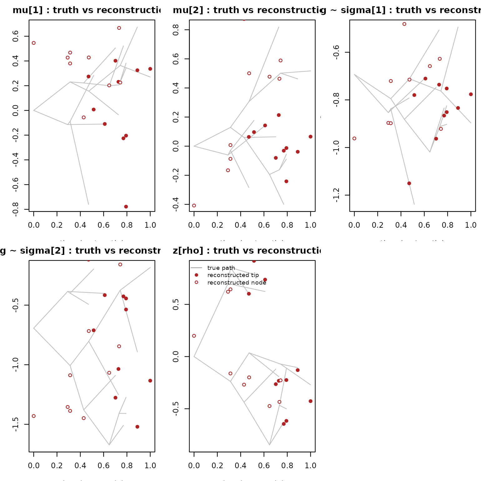
Why the reconstructed path does not look like the true path
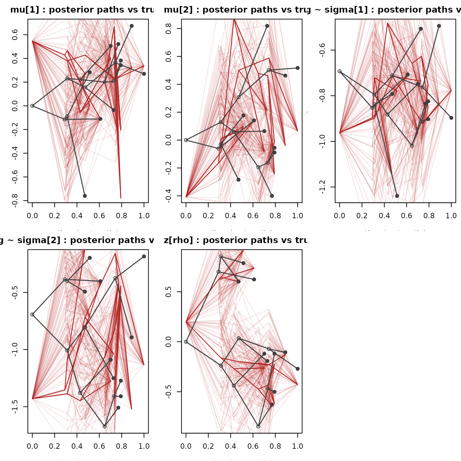
The comparison above looks disappointing if read as “the point estimate should trace the simulated path” – but that is the wrong expectation. The GLS estimator is a conditional mean: it is the smoothed compromise that minimizes squared error, not a draw from the process. A realized Brownian path is jagged; its conditional mean is not. The honest object is the posterior over the node states, which is closed-form under BM: with a flat prior on the root (the GLS estimate is the posterior mean),
So instead of one wrong-looking path we report the posterior ensemble: draws from the joint conditional are genuine Brownian-bridge paths through the fitted tips, and the true path should look like a plausible member of that ensemble. The checkable criterion is coverage, not pointwise similarity.
# posterior path draws for each parameter block
block_specs <- list(
  list(fit_mu[, 1], pr$mu_anc[1],        pr$rate_mu[1]),
  list(fit_mu[, 2], pr$mu_anc[2],        pr$rate_mu[2]),
  list(fit_ls[, 1], pr$log_sigma_anc[1], pr$rate_ls[1]),
  list(fit_ls[, 2], pr$log_sigma_anc[2], pr$rate_ls[2]),
  list(fit_zr,      pr$z_rho_anc,        pr$rate_rho))
set.seed(9); n_draw <- 40
node_draws <- lapply(block_specs, function(bs) {
  rj <- recon_joint(bs[[1]], bs[[2]], bs[[3]])
  L  <- t(chol(rj$cov))
  rj$mean + L %*% matrix(rnorm(length(nr_ids) * n_draw),
                         length(nr_ids), n_draw)
})
par(mfrow = c(2, 3), mar = c(3.2, 3.2, 2.2, 0.6))
for (i in seq_along(panels)) {
  x <- panels[[i]][[1]]
  plot(depth, x, pch = NA, xlab = "time (root -> tip)",
       ylab = panels[[i]][[2]],
       main = paste(panels[[i]][[2]], ": posterior paths vs truth"))
  for (d in seq_len(n_draw)) {                 # posterior path ensemble
    v <- fitted_all[[i]]                       # tips + mean path as base
    v[nr_ids] <- node_draws[[i]][, d]          # draw non-root nodes
    for (e in seq_len(nrow(tr$edge)))
      segments(depth[tr$edge[e, 1]], v[tr$edge[e, 1]],
               depth[tr$edge[e, 2]], v[tr$edge[e, 2]],
               col = adjustcolor("firebrick", alpha.f = 0.13))
  }
  for (e in seq_len(nrow(tr$edge)))            # posterior mean path
    segments(depth[tr$edge[e, 1]], fitted_all[[i]][tr$edge[e, 1]],
             depth[tr$edge[e, 2]], fitted_all[[i]][tr$edge[e, 2]],
             col = "firebrick", lwd = 1.2)
  for (e in seq_len(nrow(tr$edge)))            # true path on top
    segments(depth[tr$edge[e, 1]], x[tr$edge[e, 1]],
             depth[tr$edge[e, 2]], x[tr$edge[e, 2]],
             col = "grey25", lwd = 1.4)
  points(depth, x, pch = ifelse(seq_along(x) <= S, 19, 21),
         col = "grey25")
}
# 95% band coverage of the true NON-ROOT node values (the root's
# conditional sd is zero by construction -- its estimate is mu_anc,
# whose error we report directly)
true_nodes <- cbind(node_val$mu[node_ids, ], node_val$ls[node_ids, ],
                    node_val$zr[node_ids, ])
sd_nodes <- sapply(seq_along(block_specs), function(i)
  sqrt(diag(recon_joint(block_specs[[i]][[1]], block_specs[[i]][[2]],
                        block_specs[[i]][[3]])$cov)))
in_band <- abs(rec[-1, ] - true_nodes[-1, ]) <= 1.96 * sd_nodes
data.frame(parameter = c("mu1", "mu2", "ls1", "ls2", "zr"),
           node_sd = round(colMeans(sd_nodes), 3),
           coverage_95 = unname(colMeans(in_band)),
           row.names = NULL)
#>   parameter node_sd coverage_95
#> 1       mu1   0.329           1
#> 2       mu2   0.308           1
#> 3       ls1   0.289           1
#> 4       ls2   0.325           1
#> 5        zr   0.317           1
cat("root: estimate vs truth |",
    "|mu_anc - truth| =", round(abs(pr$mu_anc - truth_anc$mu), 3),
    " |ls_anc - truth| =", round(abs(pr$log_sigma_anc - truth_anc$ls), 3),
    " |zr_anc - truth| =", round(abs(pr$z_rho_anc - truth_anc$zr), 3), "\n")
#> root: estimate vs truth | |mu_anc - truth| = 0.007 0.097  |ls_anc - truth| = 0.087 0.018  |zr_anc - truth| = 0.199
Now the true paths (grey) sit inside the posterior path bundle (red) — which is the meaningful notion of correspondence. Two honest caveats: the bands inherit the inflated fitted rate (), so they are conservative (nominal 95% covering at 100%); and they condition on the fitted tip values, ignoring tip uncertainty.
The full Bayesian version runs the joint Stan model
(niche_bm_evolving_sigma) on this dataset and pushes each
posterior draw through the same conditional formula, marginalizing over
hyperparameter and tip uncertainty. On KU HPC (job 29921878, 2
chains, 2000 draws, zero divergences) the marginal node bands come out
narrower, not wider: mean sd ≈ 0.19 vs ≈ 0.31, with
coverage 0.89–1.00 across the eight non-root nodes — nearly nominal
rather than conservative. The reason is instructive: the posterior rate
(–0.7,
against a truth of 0.4–0.5) is far less inflated than the MAP corner
(–1.9),
so the full posterior partially cures the rate inflation that
made the analytic bands over-wide. Point estimates barely move (node
RMSE 0.07–0.21 in both) — what the posterior buys is calibrated
uncertainty, not better means. Draws and analyzer live in
validation/bmrt/ of the paper repository.
The levers that actually shrink node bands are structural, not computational: denser tip sampling (shorter average tip-to-node distance), more occurrences per species (tighter fitted tips), or fossil/ancient data that puts observations at the nodes themselves.
6. Round-trip summary
data.frame(
  parameter = c("mu_anc[1]", "mu_anc[2]", "ls_anc[1]", "ls_anc[2]",
                "zr_anc", "rate_mu1", "rate_mu2", "rate_ls1",
                "rate_ls2", "rate_rho"),
  truth = c(truth_anc$mu, truth_anc$ls, truth_anc$zr,
            rates$mu, rates$ls, rates$zr),
  MAP   = round(unname(c(pr$mu_anc, pr$log_sigma_anc, pr$z_rho_anc,
                  pr$rate_mu, pr$rate_ls, pr$rate_rho)), 3))
#>    parameter      truth    MAP
#> 1  mu_anc[1]  0.0000000  0.007
#> 2  mu_anc[2]  0.0000000  0.097
#> 3  ls_anc[1] -0.6931472 -0.780
#> 4  ls_anc[2] -0.6931472 -0.711
#> 5     zr_anc  0.0000000  0.199
#> 6   rate_mu1  0.5000000  1.596
#> 7   rate_mu2  0.5000000  1.395
#> 8   rate_ls1  0.4000000  1.226
#> 9   rate_ls2  0.4000000  1.552
#> 10  rate_rho  0.5000000  1.483
cat("tip mu RMSE   :", round(sqrt(mean((fit_mu - true_mu)^2)), 3), "\n")
#> tip mu RMSE   : 0.04
cat("tip ls  RMSE  :", round(sqrt(mean((fit_ls - node_val$ls[1:S, ])^2)), 3), "\n")
#> tip ls  RMSE  : 0.077
cat("tip zr  RMSE  :", round(sqrt(mean((fit_zr - node_val$zr[1:S, ])^2)), 3), "\n")
#> tip zr  RMSE  : 0.101
node_rmse <- sqrt(rowMeans((rec - cbind(node_val$mu[node_ids, ],
                                       node_val$ls[node_ids, ],
                                       node_val$zr[node_ids, ]))^2))
cat("node RMSE (mu1 mu2 ls1 ls2 zr):\n"); print(round(node_rmse, 3))
#> node RMSE (mu1 mu2 ls1 ls2 zr):
#> [1] 0.107 0.063 0.113 0.059 0.150 0.248 0.086 0.178 0.172
plot(env_grid, pch = ".", col = "grey95", main = "ancestral niche: truth vs MAP",
     xlab = "bio1", ylab = "bio12")
lines(niche_ellipse(truth_anc$mu, exp(truth_anc$ls), tanh(truth_anc$zr)),
      col = "grey30", lwd = 2)
lines(niche_ellipse(pr$mu_anc, exp(pr$log_sigma_anc), tanh(pr$z_rho_anc)),
      col = "firebrick", lwd = 2, lty = 2)
legend("topright", c("true root niche", "reconstructed root niche"),
       col = c("grey30", "firebrick"), lty = c(1, 2), lwd = 2, bty = "n")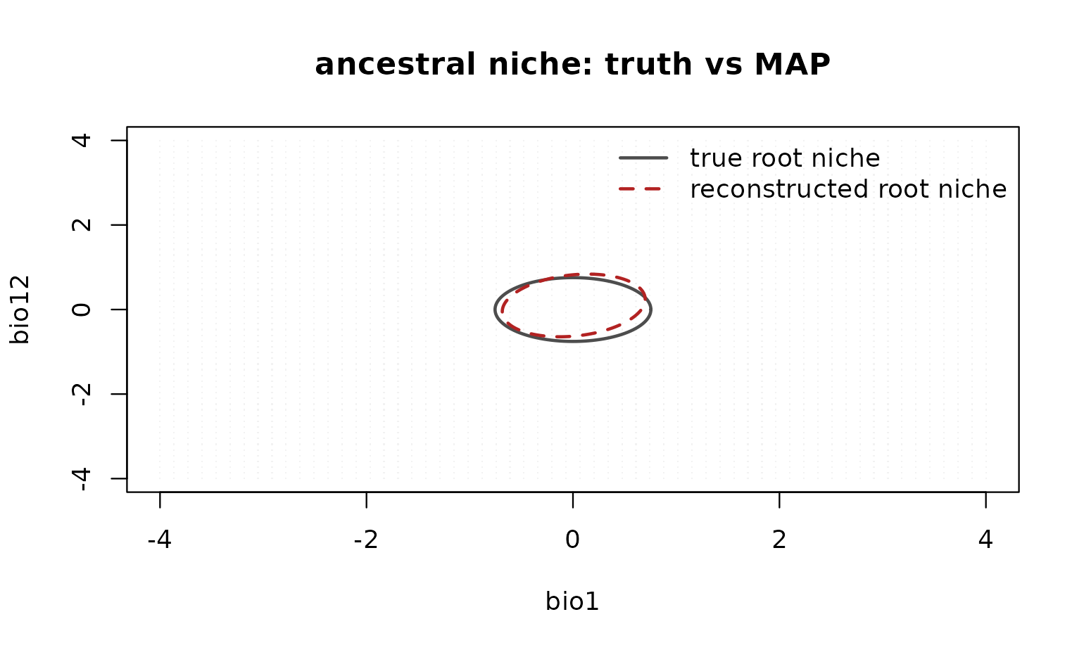
7. Same trip under an OU process
BM wanders without bound. The alternative the package implements is Ornstein–Uhlenbeck: each parameter is pulled toward an optimum with strength ,
the same transition simulate_niche_evolution() uses
under process = "ou". We rerun the trip on the
same tree with the same rates,
per block (half-life
on a unit-height tree — attraction is clearly visible), optimum
and a stationary start (root value
).
theta_ou <- list(mu = c(0.4, -0.3), ls = log(c(0.6, 0.4)), zr = 0.3)
alpha_ou <- list(mu = c(2.5, 2.5), ls = c(2.5, 2.5), zr = 2.5)

evolve_ou <- function(tree, anc, rates, alpha, theta) {
  edge <- tree$edge; el <- tree$edge.length
  n_tot <- length(tree$tip.label) + tree$Nnode
  val <- list(mu = matrix(NA_real_, n_tot, 2),
              ls = matrix(NA_real_, n_tot, 2),
              zr = matrix(NA_real_, n_tot, 1))
  val$mu[S + 1, ] <- anc$mu; val$ls[S + 1, ] <- anc$ls
  val$zr[S + 1, ] <- anc$zr
  for (e in order(edge[, 1])) {
    pa <- edge[e, 1]; ch <- edge[e, 2]; t <- el[e]
    for (b in names(val)) {
      a <- alpha[[b]]
      m <- theta[[b]] + (val[[b]][pa, ] - theta[[b]]) * exp(-a * t)
      v <- rates[[b]] / (2 * a) * (-expm1(-2 * a * t))
      val[[b]][ch, ] <- m + rnorm(ncol(val[[b]]), 0, sqrt(v))
    }
  }
  val
}

set.seed(73)
node_val_ou <- evolve_ou(tr, theta_ou, rates, alpha_ou, theta_ou)
true_mu_ou    <- node_val_ou$mu[1:S, ]
true_sigma_ou <- exp(node_val_ou$ls[1:S, ])
true_rho_ou   <- tanh(node_val_ou$zr[1:S, ])
theta_flat <- c(theta_ou$mu, theta_ou$ls, theta_ou$zr)
par(mfrow = c(2, 3), mar = c(3.2, 3.2, 2.2, 0.6))
panels_ou <- list(list(node_val_ou$mu[, 1], expression(mu[1])),
                  list(node_val_ou$mu[, 2], expression(mu[2])),
                  list(node_val_ou$ls[, 1], expression(log~sigma[1])),
                  list(node_val_ou$ls[, 2], expression(log~sigma[2])),
                  list(node_val_ou$zr[, 1], expression(z[rho])))
for (i in seq_along(panels_ou)) {
  x <- panels_ou[[i]][[1]]
  plot(depth, x, pch = NA, xlab = "time (root -> tip)",
       ylab = panels_ou[[i]][[2]],
       main = paste("true OU trajectory:", panels_ou[[i]][[2]]))
  abline(h = theta_flat[i], lty = 2, col = "steelblue", lwd = 1.5)
  for (e in seq_len(nrow(tr$edge)))
    segments(depth[tr$edge[e, 1]], x[tr$edge[e, 1]],
             depth[tr$edge[e, 2]], x[tr$edge[e, 2]], col = "grey60")
  points(depth, x, pch = ifelse(seq_along(x) <= S, 19, 21),
         col = "grey30")
}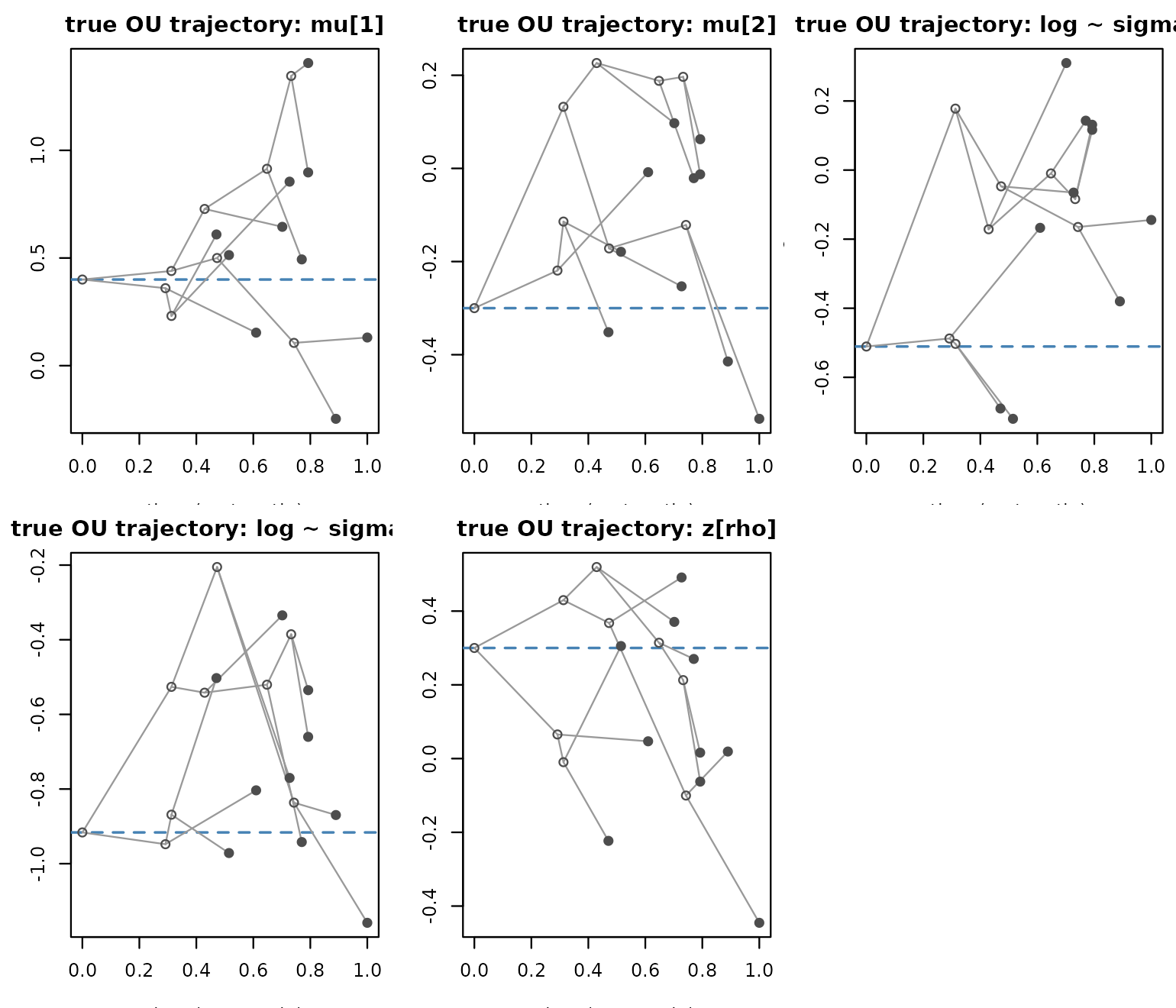
Compare with the BM traitgram above: instead of a widening fan, OU paths oscillate around the dashed optimum — the “hedgehog” signature. Tip spread is bounded by the stationary variance , not by tree height.
The misspecified trip: fitting BM to OU data
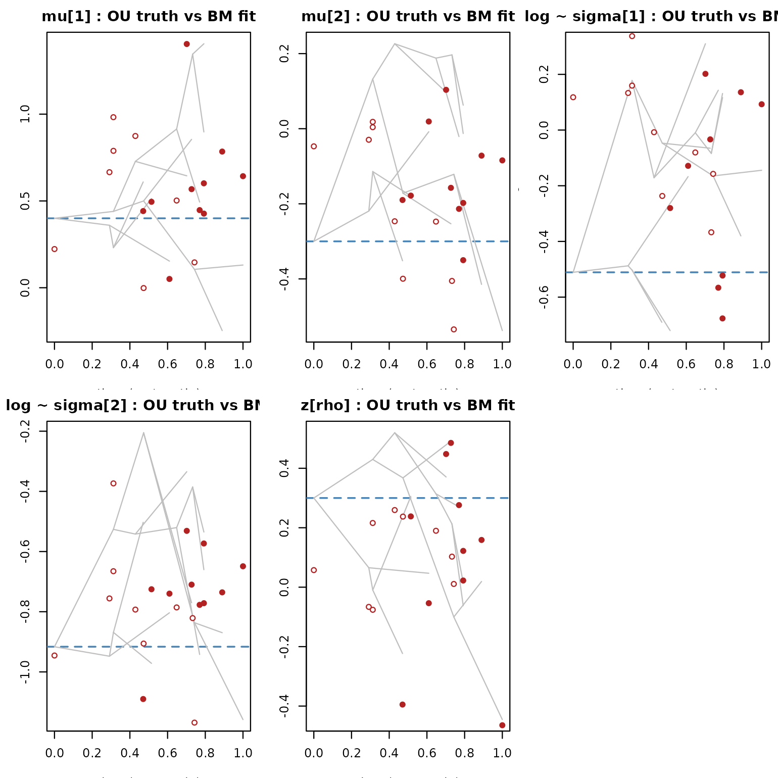
Now generate occurrences exactly as before and fit — deliberately — the BM joint MAP (the only process the local optimizer implements; the OU model is a Stan/CmdStan fit). This is the paper’s failure mode F3, process misspecification, in miniature.
occ_ou <- lapply(seq_len(S), function(s)
  virtual_species_occurrences(env_grid, mu = true_mu_ou[s, ],
                              sigma = true_sigma_ou[s, ],
                              rho = true_rho_ou[s], n_occ = 150))
names(occ_ou) <- tr$tip.label

dat_ou <- prepare_phylo_niche_data(occ_ou, bg_list, tr)
fit_ou <- niche_multistart(dat_ou, "noncentered_bounded",
                           n_starts = 8, seed = 7, verbose = FALSE)
fit_ou
#> niche_multistart (bnd)
#>   species: 10 | masked: 0
#>   map lp: -8047.85 | solutions: 8

pr_ou <- arfun:::.niche_unpack(fit_ou$map, S, P, "bnd")
fmu_ou <- sapply(1:P, function(k)
  pr_ou$mu_anc[k] + sqrt(pr_ou$rate_mu[k]) * (L_C %*% pr_ou$mu_raw[, k]))
fls_ou <- sapply(1:P, function(k)
  pr_ou$log_sigma_anc[k] + sqrt(pr_ou$rate_ls[k]) *
    (L_C %*% pr_ou$log_sigma_raw[, k]))
fzr_ou <- as.numeric(pr_ou$z_rho_anc +
                     sqrt(pr_ou$rate_rho) * (L_C %*% pr_ou$z_rho_raw))
rec_ou <- lapply(node_ids, function(a) c(
  mu = sapply(1:P, function(k) recon_node(fmu_ou[, k], pr_ou$mu_anc[k], a)),
  ls = sapply(1:P, function(k) recon_node(fls_ou[, k], pr_ou$log_sigma_anc[k], a)),
  zr = recon_node(fzr_ou, pr_ou$z_rho_anc, a)))
rec_ou <- do.call(rbind, rec_ou)

fitted_ou <- list(
  rbind(fmu_ou[, 1], rec_ou[, 1]), rbind(fmu_ou[, 2], rec_ou[, 2]),
  rbind(fls_ou[, 1], rec_ou[, 3]), rbind(fls_ou[, 2], rec_ou[, 4]),
  c(fzr_ou, rec_ou[, 5]))
#> Warning in rbind(fmu_ou[, 1], rec_ou[, 1]): number of columns of result is not
#> a multiple of vector length (arg 2)
#> Warning in rbind(fmu_ou[, 2], rec_ou[, 2]): number of columns of result is not
#> a multiple of vector length (arg 2)
#> Warning in rbind(fls_ou[, 1], rec_ou[, 3]): number of columns of result is not
#> a multiple of vector length (arg 2)
#> Warning in rbind(fls_ou[, 2], rec_ou[, 4]): number of columns of result is not
#> a multiple of vector length (arg 2)
par(mfrow = c(2, 3), mar = c(3.2, 3.2, 2.2, 0.6))
for (i in seq_along(panels_ou)) {
  x <- panels_ou[[i]][[1]]
  plot(depth, x, pch = NA, xlab = "time (root -> tip)",
       ylab = panels_ou[[i]][[2]],
       main = paste(panels_ou[[i]][[2]], ": OU truth vs BM fit"))
  abline(h = theta_flat[i], lty = 2, col = "steelblue", lwd = 1.5)
  for (e in seq_len(nrow(tr$edge)))
    segments(depth[tr$edge[e, 1]], x[tr$edge[e, 1]],
             depth[tr$edge[e, 2]], x[tr$edge[e, 2]], col = "grey75")
  points(depth[1:S], fitted_ou[[i]][1:S], pch = 19,
         col = "firebrick", cex = 0.9)
  points(depth[node_ids], fitted_ou[[i]][S + 1:tr$Nnode],
         pch = 21, bg = "white", col = "firebrick", cex = 0.9)
}
data.frame(
  parameter = c("mu_anc[1]", "mu_anc[2]", "ls_anc[1]", "ls_anc[2]",
                "zr_anc", "rate_mu1", "rate_mu2", "rate_ls1",
                "rate_ls2", "rate_rho"),
  theta_or_truth = c(theta_ou$mu, theta_ou$ls, theta_ou$zr,
                     rates$mu, rates$ls, rates$zr),
  BM_MAP_on_OU = round(unname(c(pr_ou$mu_anc, pr_ou$log_sigma_anc,
                                pr_ou$z_rho_anc, pr_ou$rate_mu,
                                pr_ou$rate_ls, pr_ou$rate_rho)), 3))
#>    parameter theta_or_truth BM_MAP_on_OU
#> 1  mu_anc[1]      0.4000000        0.495
#> 2  mu_anc[2]     -0.3000000       -0.178
#> 3  ls_anc[1]     -0.5108256       -0.280
#> 4  ls_anc[2]     -0.9162907       -0.725
#> 5     zr_anc      0.3000000        0.057
#> 6   rate_mu1      0.5000000        1.888
#> 7   rate_mu2      0.5000000        1.171
#> 8   rate_ls1      0.4000000        1.337
#> 9   rate_ls2      0.4000000        1.359
#> 10  rate_rho      0.5000000        1.447
cat("tip mu RMSE (OU data, BM fit):",
    round(sqrt(mean((fmu_ou - true_mu_ou)^2)), 3), "\n")
#> tip mu RMSE (OU data, BM fit): 0.086
Three things to read off the misspecified fit:
- Tip values still land correctly — the occurrence clouds pin them down regardless of the process prior; tip RMSE stays small.
- The root estimate lands near θ anyway: under stationary OU the tips cluster around the optimum, so the BM weighted-mean reconstruction lands close to θ — a correct point estimate for the wrong reason. What it cannot express is the regression-to-θ geometry of the true paths.
-
The rates are uninterpretable: the BM layer reads
both the bounded stationary spread and per-species estimation
noise as diffusion, inflating
rate_*roughly threefold — the same noise-soaking mechanism as the correctly specified BM run — and there is no slot where the attraction could be reported. The fitted “process” is fiction: OU’s pull is silently rewritten as a featureless diffusion.
The correct-fit path is the OU Stan model:
fit_evolution(stan_data, model = "ou_evolving") fits the
joint occurrence + OU likelihood with
and
as free parameters (the mu_anc parameter doubles as the
optimum θ). For this exact dataset that model was run on KU HPC (CmdStan
2.36, SLURM job 29921840, 2 chains, 1000 warmup + 1000 sampling, 2
divergences, all
).
Posterior medians for the attraction strength:
,
,
— all against a truth of 2.5, with wide 90% intervals (roughly 0.2–6.6):
is weakly identified with ten tips but the posterior is centred
correctly and, unlike the BM fit, the parameter exists to be
estimated. The variance parameters
come out inflated (medians
,
,
against truths of 0.25, 0.16, 0.25) — the same noise-absorption
mechanism as the BM rates. Draws, diagnostics and the analyzer live in
validation/ou/ of the paper repository. The point of the
contrast: the right process estimates the attraction, the wrong
process hides it inside an inflated rate — which is why the paper
insists on reporting the fitted process alongside any ancestral
reconstruction.
What to look at
- Centroids () are the best-identified parameters: occurrence clouds locate them directly, and node reconstructions track the true path closely.
- Log tolerances and are noisier at the tips (a presence cloud pins down an ellipse’s shape weakly) but the BM prior pools information across the tree – the phylogeny is doing measurable work.
- Rates (, , ) are the hardest: with ten tips the likelihood carries little information about variance parameters, so MAP rates sit inside wide priors. In this run they come out inflated roughly threefold – the raw deviations soak up per-species estimation noise, which the BM layer then reads as rate. Treat them as order-of-magnitude statements.
- The residual caveats of the pipeline apply: this is a MAP fit, not a posterior; is the oracle uniform-over-domain case; and .