Your own data: from a tree, occurrences, and climate rasters to ancestral niches

The round-trip vignette simulates everything. This one starts where most users start: you already have data – a phylogeny, a table of occurrence points, and climate rasters – and you want to reconstruct the evolution of the niche over the clade.

The example is a real clade bundled with the package: six Vulpes foxes, GBIF occurrences, an ERA5-Land bioclimatic window, and per-species accessible-area polygons derived from ecoregions. The files are small and live in inst/extdata/vulpes/ – and each one comes from a public service, so the same recipe works for your own clade:

climate: yearly ERA5-Land bioclim GeoTIFFs from https://bioclim.ecoseek.org (/api/download/{year}/{var}_{year}.tif), averaged over 1991–2020 – the bundled vulpes_climate.tif is that product cropped and coarsened;
accessible areas: oneearthr::oe_layer("ecoregions") (RESOLVE Ecoregions 2017) – each species’ $M_s$ is the dissolved union of the ecoregions containing its occurrences;
occurrences/tree: GBIF + VertLife, frozen into the bundle;
prior ellipses: xnicher::optimize_niche per species, wrapped by niche_warmstart().

The runnable recipe is data-raw/vulpes_bundle.R in the source tree; the retrieval steps are shown below where they belong in the workflow.

What arfun consumes (and what it does not)

arfun does not read coordinates or rasters in the fitting functions. The joint niche-evolution model consumes three things:

a phylo tree whose tip labels match your species names;
env_occ_list: a named list with one numeric matrix per species of environmental values already extracted at that species’ occurrence points (rows = points, columns = variables);
env_m_list: the same, but for a sample of the accessible environmental background $M_s$ of each species.

Everything else – reading files, intersecting points with rasters, deciding what $M_s$ is – is user-side work, and that is the honest division of labour: those choices are scientific decisions, not plumbing. This vignette walks through them.

1. Read the inputs

library(arfun)
library(ape)      # read.tree
library(terra)    # rast, vect, extract
#> terra 1.9.50
#> 
#> Attaching package: 'terra'
#> The following objects are masked from 'package:ape':
#> 
#>     rotate, trans, zoom

extdata <- system.file("extdata/vulpes", package = "arfun")
# when working from the source tree:
# extdata <- "inst/extdata/vulpes"

tree   <- read.tree(file.path(extdata, "vulpes_tree.nwk"))
occ    <- read.csv(file.path(extdata, "vulpes_occurrences.csv"))
clim   <- rast(file.path(extdata, "vulpes_climate.tif"))   # bio01, bio12
m_poly <- vect(file.path(extdata, "vulpes_m_polygons.gpkg"))

tree
#> 
#> Phylogenetic tree with 6 tips and 5 internal nodes.
#> 
#> Tip labels:
#>   Vulpes_pallida, Vulpes_macrotis, Vulpes_velox, Vulpes_corsac, Vulpes_bengalensis, Vulpes_chama
#> 
#> Rooted; includes branch length(s).
head(occ)
#>              species      lon      lat
#> 1 Vulpes bengalensis 78.17069 26.77858
#> 2 Vulpes bengalensis 77.32323 13.74005
#> 3 Vulpes bengalensis 85.45174 20.20224
#> 4 Vulpes bengalensis 73.80882 17.72114
#> 5 Vulpes bengalensis 88.78066 26.33454
#> 6 Vulpes bengalensis 71.28742 23.46182
clim
#> class       : SpatRaster
#> size        : 227, 522, 2  (nrow, ncol, nlyr)
#> resolution  : 0.5, 0.5  (x, y)
#> extent      : -128.55, 132.45, -40.15, 73.35  (xmin, xmax, ymin, ymax)
#> coord. ref. : lon/lat WGS 84 (EPSG:4326)
#> source      : vulpes_climate.tif
#> names       :      bio01,         bio12
#> min values  : 245.087204,             0
#> max values  : 306.367157, 221473.140625

Real files never align on the first try. The VertLife-derived tip labels carry underscores; the occurrence table uses spaces:

tree$tip.label <- gsub("_", " ", tree$tip.label)
stopifnot(all(occ$species %in% tree$tip.label))
plot(tree, main = "Vulpes clade"); axisPhylo()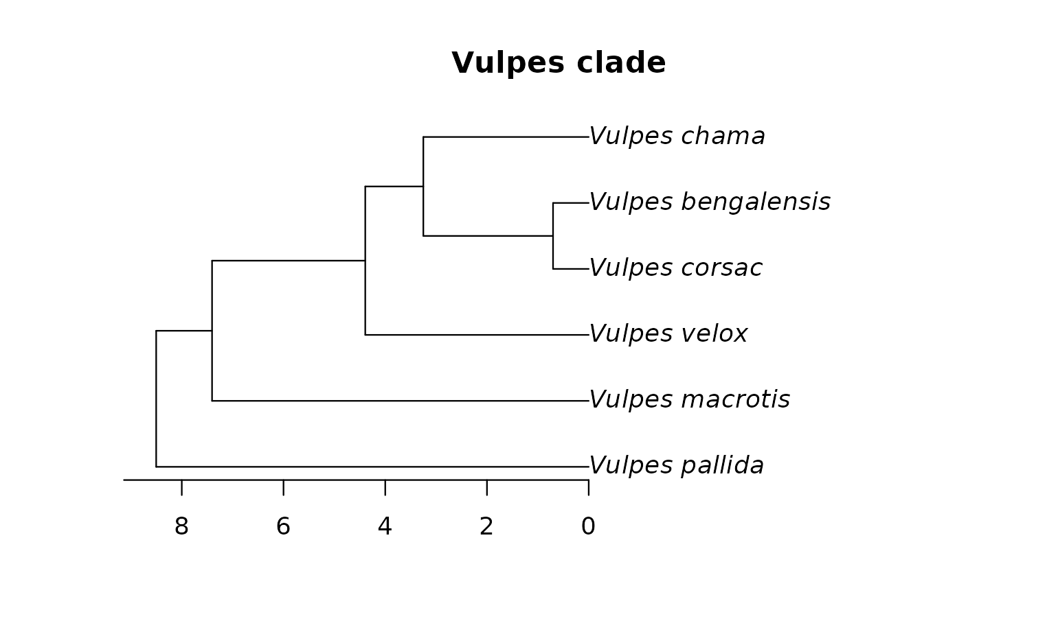

2. Extract climate at the occurrence points

The bundled raster came from bioclim.ecoseek.org; for your own clade the download is two lines per variable-year:

years <- 1991:2020
url <- function(v, y) sprintf(
  "https://bioclim.ecoseek.org/api/download/%d/%s_%d.tif", y, v, y)
stk <- rast(vapply(years, function(y) {
  f <- tempfile(fileext = ".tif")
  download.file(url("bio01", y), f, mode = "wb", quiet = TRUE); f
}, character(1)))
bio01_mean <- mean(stk)   # climatology: average the yearly fields

terra::extract pulls the raster values at each coordinate. arfun then wants one matrix per species, in a named list, with names equal to the tip labels:

pts <- vect(occ, geom = c("lon", "lat"), crs = "EPSG:4326")
env_at_occ <- extract(clim, pts, ID = FALSE)

env_occ_list <- split(as.data.frame(env_at_occ), occ$species)
env_occ_list <- lapply(env_occ_list,
                       function(x) as.matrix(x[complete.cases(x), ]))
sapply(env_occ_list, nrow)
#> Vulpes bengalensis       Vulpes chama      Vulpes corsac    Vulpes macrotis 
#>                178                193                187                672 
#>     Vulpes pallida       Vulpes velox 
#>                  1                300

3. Standardize the environmental axes

bio01 arrives in tenths of kelvin and bio12 in mm of precipitation; the model works on any units, but comparable scales make priors meaningful and rates interpretable. Standardize with the clade-pooled occurrence moments (so every species shares the same units), and keep the constants: you need them again to interpret parameters or project back.

all_occ <- do.call(rbind, env_occ_list)
mu0 <- colMeans(all_occ)
sd0 <- apply(all_occ, 2, sd)
env_occ_list <- lapply(env_occ_list, function(x) scale(x, mu0, sd0))

4. Declare M: the accessible background

This is the step the paper stresses: the likelihood normalizes each species’ niche against the environments it could plausibly have reached. The bundled polygons declare $M_s$ as the dissolved union of RESOLVE ecoregions containing that species’ records, built with oneearthr (shipped offline, no download needed at scale = "small"):

library(oneearthr)
eco <- oe_layer("ecoregions")                # or "bioregions"/"realms"
hit <- relate(eco, pts, "intersects")
m_of <- function(s)
  aggregate(eco[rowSums(hit[, occ$species == s, drop = FALSE]) > 0, ])
m_poly <- do.call(rbind, lapply(tree$tip.label, function(s) {
  m <- m_of(s); m$species <- s; m
}))

Choosing oe_layer("realms") or "bioregions" instead changes the declared accessible domain – deliberately coarser $M$ hypotheses, useful as sensitivity analyses. Sample background points inside each polygon:

bg_list <- lapply(seq_len(nrow(m_poly)), function(i) {
  clim_m <- mask(crop(clim, m_poly[i]), m_poly[i])
  s <- spatSample(clim_m, size = 2000, method = "regular",
                  na.rm = TRUE, warn = FALSE)
  as.matrix(s[complete.cases(s), ])
})
names(bg_list) <- m_poly$species
bg_list <- lapply(bg_list, function(x) scale(x, mu0, sd0))
sapply(bg_list, nrow)
#>     Vulpes pallida    Vulpes macrotis       Vulpes velox      Vulpes corsac 
#>                633               1118               1270                784 
#> Vulpes bengalensis       Vulpes chama 
#>                967                877

If all species share one accessible domain, draw a single sample and pass the identical matrix to every species – shared_background_sample() exists for that. Independent subsamples of a shared $M$ create Monte Carlo “holes” that leak likelihood into a spurious $\sigma \to 0$ mode.

5. Sparse species: `mask_species`

Presence-only data bound the niche from above; a species with a handful of points carries essentially no shape information. Look at the counts: Vulpes pallida has 1 usable point – not enough to identify an ellipse. mask_species keeps it in the phylogenetic prior but drops it from the likelihood, so its niche is predicted from its relatives – an identifiability limit turned into a testable prediction.

sparse <- names(which(sapply(env_occ_list, nrow) < 10))
sparse
#> [1] "Vulpes pallida"

stan_data <- prepare_phylo_niche_data(
  env_occ_list, bg_list, tree, mask_species = sparse)
str(stan_data[c("S", "P", "N_occ_total", "N_m_total", "masked")])
#> List of 5
#>  $ S          : int 6
#>  $ P          : int 2
#>  $ N_occ_total: int 1530
#>  $ N_m_total  : int 5016
#>  $ masked     : logi [1:6] TRUE FALSE FALSE FALSE FALSE FALSE

6. Prior ellipses: per-species `xnicher` fits

Before the joint model, fit each species on its own. niche_warmstart() runs xnicher::optimize_niche() (CRAN) per species against its declared $M_s$ , keeps the fits that avoid the degenerate $\sigma \to 0$ mode, and assembles a starting vector for the joint parameterization – unfitted or masked species start at the phylogenetic conditional mean of the fitted ones:

warm <- niche_warmstart(stan_data)
warm$per_species
#>              species fitted n_cells         mu1        mu2    sigma1    sigma2
#> 1     Vulpes pallida  FALSE       0 -0.29376559  0.7417480 0.7274098 0.7435732
#> 2    Vulpes macrotis   TRUE     243  0.56388797 -0.7625873 0.6995400 0.3787386
#> 3       Vulpes velox   TRUE     148 -0.36619290  0.1401475 0.5308045 0.3906080
#> 4      Vulpes corsac   TRUE     138 -2.34274925 -0.2000157 1.4376602 0.5738216
#> 5 Vulpes bengalensis   TRUE      99  0.70539170  4.8943601 0.5306238 3.0896338
#> 6       Vulpes chama   TRUE     113 -0.02916547 -0.3631646 0.7189614 0.8666707
#>          rho
#> 1 -0.3877556
#> 2 -0.7181765
#> 3 -0.3335702
#> 4  0.5700520
#> 5 -0.6902180
#> 6 -0.5209834

per_species is the interesting object on its own: the independent M-restricted niche estimate of each species, i.e. what the data would say without phylogenetic pooling. Comparing it with the joint fit below shows what the evolutionary model adds – and fitted = FALSE flags the species whose ellipse is prior-driven rather than identified.

7. Fast screen: the MAP fit

Before paying for MCMC, run niche_multistart(): a space-filling design over the joint posterior optimized with the compiled C++ objective, plus the warm-start vector so the search begins at the per-species optima. It takes seconds for a clade this size and flags boundary behaviour (collapsed/sliver/inflated niches) via niche_boundary_report():

ms <- niche_multistart(stan_data, n_starts = 16, seed = 1,
                       extra_starts = warm$theta)
#> niche_multistart: 10/17 finite starts | objective: C++ (ucminf_xptr)
#> start 17 -> lp -9886.66 conv 4 maxgrad 3.11e-03
#> start 16 -> lp -9886.66 conv 4 maxgrad 1.29e-04
#> start 13 -> lp -9898.30 conv 4 maxgrad 3.69e-04
#> start  1 -> lp -9898.30 conv 4 maxgrad 6.72e-04
#> start  4 -> lp -9886.66 conv 4 maxgrad 1.02e-03
#> start 10 -> lp -9895.02 conv 4 maxgrad 4.58e-04
#> start 14 -> lp -9886.67 conv 4 maxgrad 3.08e-02
#> start  8 -> lp -9886.66 conv 4 maxgrad 1.64e-03
#> start  2 -> lp -9929.12 conv 4 maxgrad 3.87e-04
#> start  5 -> lp -9886.66 conv 4 maxgrad 4.73e-04
#> boundary flags: Vulpes pallida:masked
ms$map_lp
#> [1] -9886.665
niche_boundary_report(stan_data, ms$map)
#>                               species    sigma1    sigma2        rho emp_sd_min
#> Vulpes pallida         Vulpes pallida 0.9068439 0.7161258 -0.3387979         NA
#> Vulpes macrotis       Vulpes macrotis 0.6311007 0.3199016 -0.7123355  0.2539716
#> Vulpes velox             Vulpes velox 0.5710128 0.3411500 -0.3803959  0.2898072
#> Vulpes corsac           Vulpes corsac 1.7005371 0.6038770  0.6214095  0.4068340
#> Vulpes bengalensis Vulpes bengalensis 0.6615082 3.6065438 -0.8860496  0.3045495
#> Vulpes chama             Vulpes chama 2.2778302 1.4980154 -0.9010711  0.3901817
#>                    n_occ n_cells masked   flag
#> Vulpes pallida         0       0   TRUE masked
#> Vulpes macrotis      672     243  FALSE     ok
#> Vulpes velox         300     148  FALSE     ok
#> Vulpes corsac        187     138  FALSE     ok
#> Vulpes bengalensis   178      99  FALSE     ok
#> Vulpes chama         193     113  FALSE     ok

Read the flags before reading the numbers. Here every fitted species reports ok – the declared $M_s$ contains enough accessible contrast to identify the ellipses – and only the masked Vulpes pallida is flagged. Contrast this with what a tighter or misspecified $M$ produces (the simulation vignette’s outside cells): the optimizer then slides along a flat ridge and the report flags at_floor/sigma_huge. Boundary flags are a diagnostic of the $M$ hypothesis, not just of the optimizer. The Bayesian fit below still matters: the MAP is a point on a ridge, and the posterior carries the mass the point estimate discards.

8. Full posterior: `fit_evolution`

The Bayesian fit samples tip niches, ancestral states, and evolutionary rates jointly. On a laptop this takes on the order of ten minutes for six tips; on a cluster, pre-compile the model once and pass it via mod =.

fit <- fit_evolution(stan_data, model = "bm_evolving",
                     chains = 2, iter_warmup = 1000,
                     iter_sampling = 1000, seed = 7,
                     mod = compile_model("bm_evolving"))

The vignette ships the result of exactly this call, run on KU HPC:

cache_file <- file.path(extdata, "vulpes_bm_evolving_cache.rds")
cache <- if (file.exists(cache_file)) readRDS(cache_file) else NULL
if (!is.null(cache)) {
  dg <- cache$diagnostics
  cat("cached fit:", cache$args$model, "| draws:", nrow(cache$draws),
      "| divergences:", sum(dg$num_divergent),
      "| max-treedepth hits:", sum(dg$num_max_treedepth),
      "| min E-BFMI:", round(min(dg$ebfmi), 2), "\n")
}
#> cached fit: bm_evolving | draws: 2000 | divergences: 5 | max-treedepth hits: 1938 | min E-BFMI: 0.53

Report the diagnostics, not just the estimates: on this dataset 5 transitions diverge and most hit the maximum treedepth – the sampler reaches the answers but moves slowly through the funnel-shaped posterior (the phylogenetically pooled variance geometry). ESS stays above ~120 and $\hat{R} \le 1.02$ , so the marginals are usable, but a deeper treedepth or a non-centered reparameterization is the honest next step for production use.

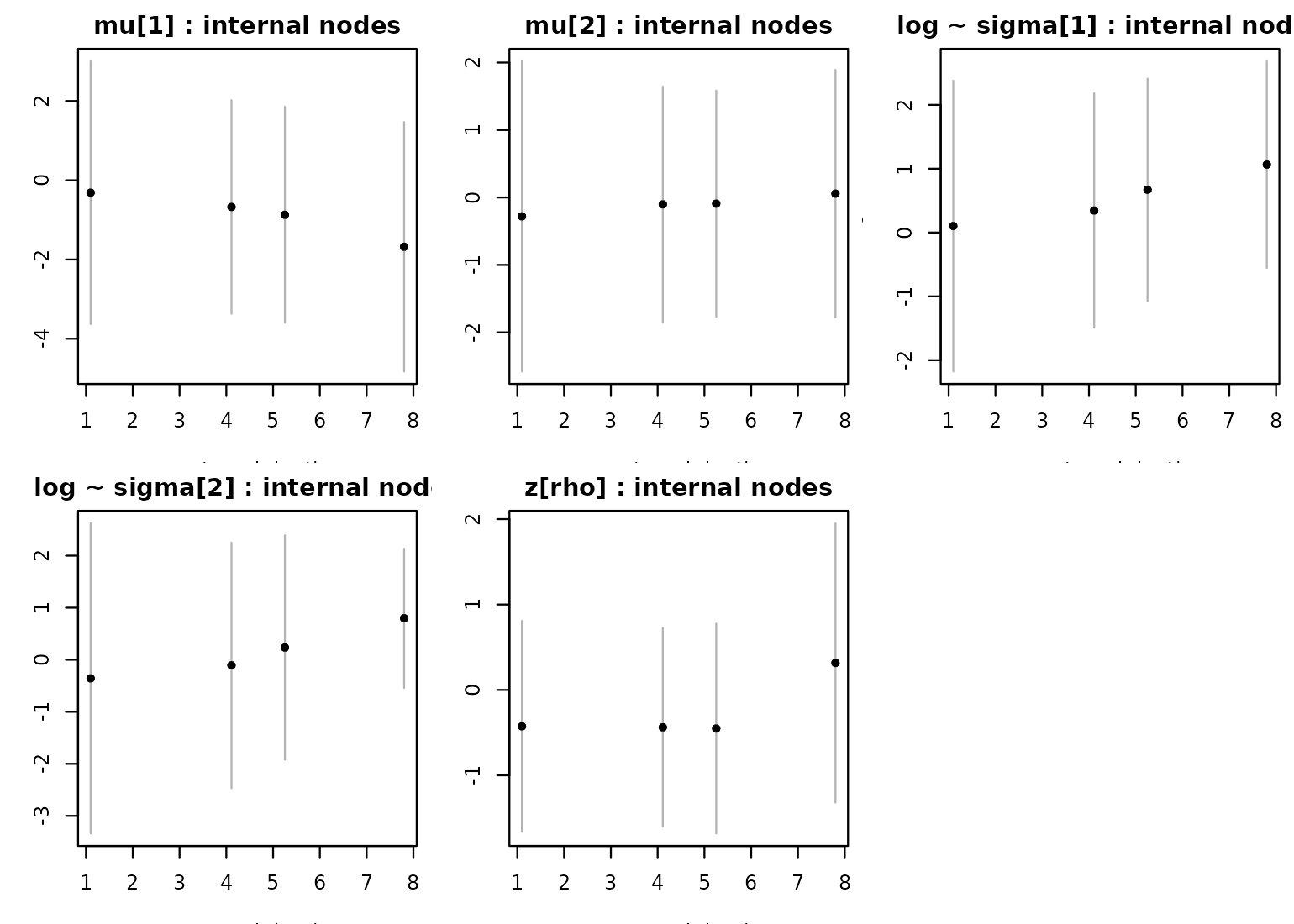
The Stan model samples tip states; internal-node posteriors are reconstructed post-hoc by pushing each draw through the BM conditional formula – $\mathbb{E}[y_{anc}\mid y_{tips}] = \mu_{anc} + W(y_{tips} - \mu_{anc})$ with $W = V_{N,T}V_{T,T}^{-1}$ from the phylogenetic covariance. The cache already contains these marginals (cache$node_posterior); the computing recipe lives in ?prepare_phylo_niche_data and the package vignette sources.

if (!is.null(cache)) {
  np <- cache$node_posterior
  depth <- node.depth.edgelength(tree)
  par(mfrow = c(2, 3), mar = c(3.2, 3.2, 2, 0.6))
  panels <- list(list(np$mu1, expression(mu[1])),
                 list(np$mu2, expression(mu[2])),
                 list(np$ls1, expression(log~sigma[1])),
                 list(np$ls2, expression(log~sigma[2])),
                 list(np$zr,  expression(z[rho])))
  for (pn in panels) {
    m <- pn[[1]]$mean; s <- pn[[1]]$sd
    d <- depth[cache$node_ids]
    plot(d, m, pch = 19, cex = 0.7,
         xlab = "rootward depth", ylab = pn[[2]],
         ylim = range(m + 2 * s, m - 2 * s),
         main = paste(pn[[2]], ": internal nodes"))
    segments(d, m - 2 * s, d, m + 2 * s, col = "grey70")
    points(d, m, pch = 19, cex = 0.7)
  }
}

9. Back to geography

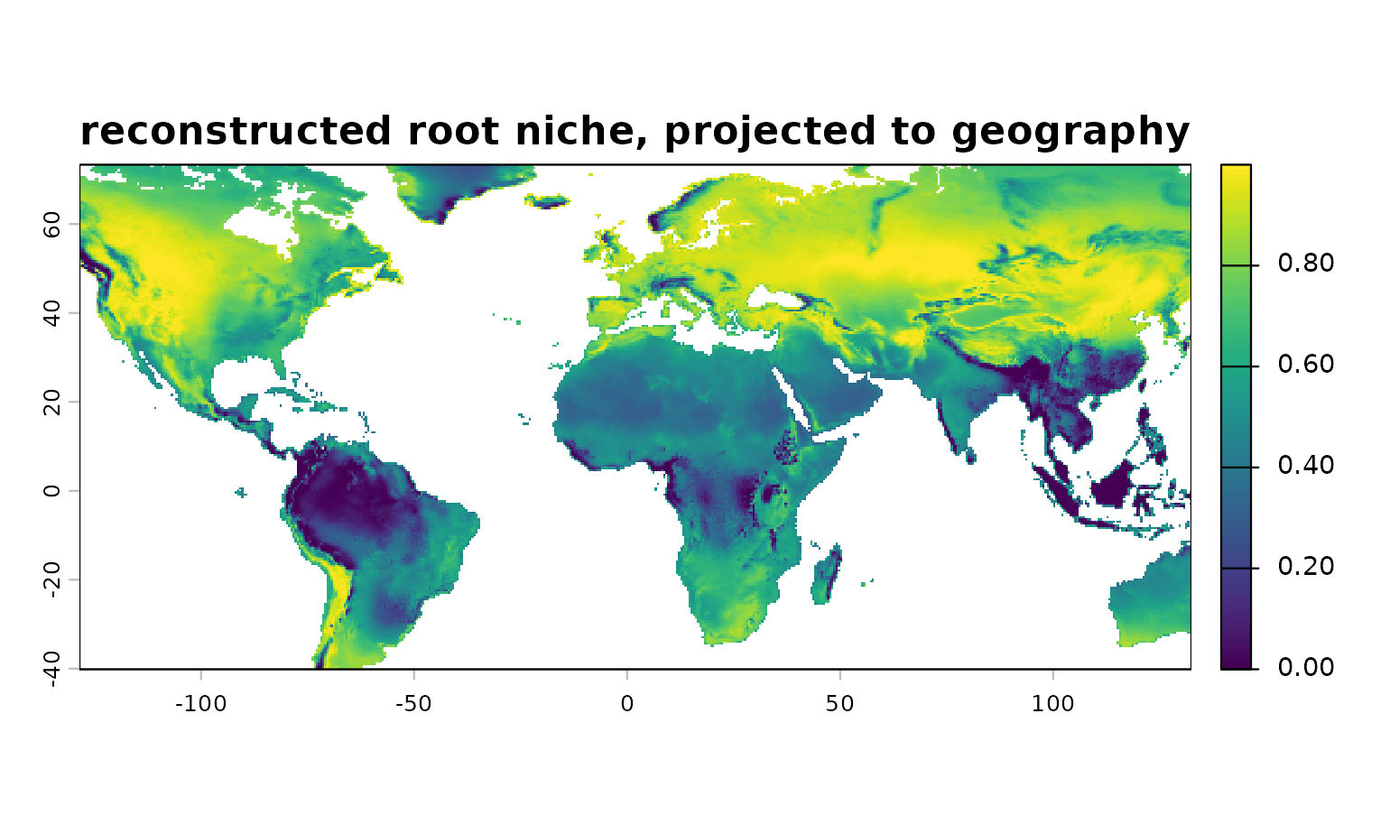
project_single_niche() evaluates the Mahalanobis suitability of any state – tip or reconstructed node – on a raster. Project the root state (un-standardizing back to raster units first, since clim is raw):

if (!is.null(cache)) {
  np <- cache$node_posterior
  root <- which.max(depth[cache$node_ids])
  mu_z  <- c(np$mu1$mean[root], np$mu2$mean[root])
  sg_z  <- c(exp(np$ls1$mean[root]), exp(np$ls2$mean[root]))
  rho   <- tanh(np$zr$mean[root])
  # un-z-score: x_raw = x_z * sd0 + mu0, so mu_raw = mu_z*sd0+mu0 and
  # Sigma_raw = D sd0 %*% Sigma_z %*% D sd0
  mu_raw <- mu_z * sd0 + mu0
  Sz <- diag(sg_z); R <- matrix(c(1, rho, rho, 1), 2)
  Sigma_raw <- diag(sd0) %*% Sz %*% R %*% Sz %*% diag(sd0)
  suit <- project_single_niche(mu_raw, Sigma_raw, clim)
  plot(suit, main = "reconstructed root niche, projected to geography")
}

Honest scope

The fitted ellipse is the niche conditioned on the declared $M_s$ – change the background and the answer changes. The round-trip vignette shows what a flat background does to coverage.
A suitability map of an ancestral state is a projection of a statistical estimate, not a paleodistribution reconstruction.
The joint evolutionary models are currently two-dimensional (bio01, bio12 here). fit_niche() (single species, no phylogeny) accepts more dimensions.
Presence-only data bound the niche from above; sparse species belong in mask_species, not in the likelihood.